
Part V: The fundamental biological groupings
V.1.1 We now have to relate the homomorphic structures biological entities can create to the homeomorphic spaces in which they must move. Since they must all recurve in a four-dimensional space, then we can enumerate their fundamental properties.
Our Commandos 1 and 2 in Figure 12 showed how to measure the populations underneath them. However, those populations can easily follow homotopic and quantitatively equivalent paths, which begin and end in the same location, but that are not qualitatively equivalent, or homeomorphic. Their 0-, 1-, 2-, and 3-balls can easily exhibit the same V1,2,3,4. But their paths across their respective S0,1,2,3 surfaces, as measured by their 0-, 1-, 2-, and 3-spheres, could be radically different. Since we currently have no way to distinguish any such paths, then we have no way to distinguish biological populations.
V.1.2 Our stases of the first, second and third kinds, and our three constraints, may each sum to zero, but they are importantly different. Since the three stases of ∇Q = ∇ • Q = ∇ × Q = 0 incorporate gradients, divergences, and curls, then they are critically dependent upon the precise paths, and directions, they each take. Since they measure surfaces, S, they are “inexact differentials”.
V.1.3 The three constraints of ∫dn = ∫dM = ∫dP = 0 present a direct contrast. They are completely indifferent to surfaces and paths. They instead measure interiors, giving values for gongyls for rotachorons, volumes for rotahedrons, areas for rotagons and the like. They depend only upon initial and final values and states. Since they measure volumes, V, they are exact differentials.
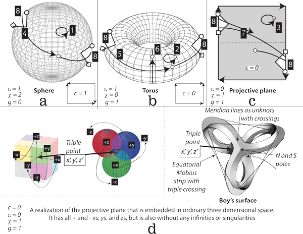
V.1.4 We can separate the three stases from the three constraints using the three sets of curves on the sphere, the torus, and the real projective plane in Figure 27. The two sets of curves may have certain topological similarities, but they nevertheless create very different paths against the three sets of ijk, IJK and TNB axes that our Frenet-Serrat trihedron can measure. Those differences will have different topological effects on each of the three types of surface, meaning different biologies.
V.1.5 Figure 27 sets us on our way by demonstrating, for Meme 119, that no populations can complete a circulation of the generations without at some time undertaking transformations—such as in the white Regions 8—that are the direct opposite of those they undertake at some other point. Those opposite points must then be the real projective plane’s identified points.
Since the four dimensions on a real projective plane are again impossible to visualize, we turn to Boy’s surface, shown in Figure 27d. It is the most accessible three-dimensional representation of a set of four-dimensional interactions.
Werner Boy discovered his realization of a real projective plane, in 1901, when his thesis supervisor, David Hilbert, challenged him to prove that one could not be realized in ordinary three-dimensional Euclidean space. As in Figure 27d, Boy successfully connected the positive x-axis to the negative y-axis, the positive y-axis to the negative z-axis, and the positive z-axis to the negative x-axis. Those twisted xy, xz, and yz planes recreate their x = 0, y = 0, and z = 0 origin by intersecting in exactly their one “triple point”.
Boy’s surface may help us investigate our biological symmetries, but since the unbounded but noninfinite realm it depicts cannot be properly realized without a fourth dimension, it is deceptive. It alludes that its three infinitely extensive Euclidean (xy)zw, (xz)yw, and (yz)xw planes are in fact circulating planespaces. It also suggests a discrete inside and outside, and so positive and negative locales, over all three of our observable dimensions. We can therefore be left with the impression that the limited realmspace at its centre is the reality … but we have not seen any w measures.
The deception in Boy’s surface is precisely that it handles events in four dimensions … and then represents them in three. We see (xyz)w but do not see (xyw)z, (xzw)y, or (yzw)x .
Boy’s surface can be both a mapping cylinder and/or a fibre bundle. However, a fibre bundle, being a product, can have either or both of its base or fibre as either or both of its projection map and retract. Either or both can contain flips, orientations, magnitudes, and rates of change independent of the other. The upshot is that two neighbourhoods can be homeomorphic, and near each other, on Boy’s surface seen as a mapping cylinder, without their equivalent neighbourhoods being either homeomorphic or near each other on either the base or the fibre that give rise to it. Populations and entities can therefore be near to each other in one structure, but appear separated in another.
The realmspace enclosed in Boy’s surface also belies reality by seemingly trapping all positive, or else all negative, neighbourhoods inside it. But as in this real and three-dimensional realm, it is, firstly, always possible to keep moving onwards infinitely, unboundedly, and rectilinearly in both the positive and the negative directions without ever circling back. And secondly, the surface’s constant curves suggest that a similarly curved tetraspace influences the Boy’s surface events. However, the tetrarealm that imposes those apparently curving x, y and z behaviours in fact extends indefinitely in all its four directions.
V.1.6 We begin by considering a one-dimensional line, x. Since biological entities are not infinite in that they must be replaced, they have the same general difficulty as all manifolds that, like Boy’s surface, are without a boundary; that are unbounded; and yet that are not infinite in extent.
A circle is a one-manifold with the local topology of an infinitely extended line, x → ±∞, but with a limited or bounded global topology. It cannot be properly built—as a one-manifold without boundary—within that same one dimensional line. We can only realize its noninfinite and unbounded global topology by creating a two-dimensional circle, (x | y). That then provides the infinitely many linespaces for all required line segments.
The circle we use to create our unbounded one-dimensional expanse adds another important possibility. Whatever direction we move in at one point on the manifold, we can move in the opposite direction at another (x | ±y). We can also eventually return to the original point or orientation. The added dimension therefore allows us to reverse orientations because we can have both (x | +y) at one moment, and (x | -y) at another, with no discernible difference in x: (x → ±∞ | ±y).
V.1.7 We then turn to two-dimensional areas, (x, y), or (x → ±∞, y → ±∞). An infinitely extended but unbounded two-dimensional plane and manifold is easy enough to visualize. We simply provide a sphere’s surface. Its local topology gives the identical impression of being infinite, even though it is of limited extent. However, that limited yet unbounded two-manifold cannot be built in those same two dimensions. We must turn to a third to construct the sphere whose surface then provides the relevant planespace as (x → ±∞, y → ±∞ | z).
Our sphere’s unbounded planespace promptly gives us the same possibility as the circle did for the line. We can soon find a local direction to move in that is counter to any current one. Our third dimension can first reverse, and then restore, any two-dimensional orientation: (x → ±∞, y → ±∞ | ±z).
V.1.8 The analogous situation holds for three (x → ±∞, y → ±∞, z → ±∞) dimensions. The surrounding cosmos gives every impression of being an ever-extending and infinite realm. But it is impossible for us to realize an unbounded and noninfinite three dimensional realmspace within these same three dimensions.
Although we now know that the surrounding universe supports the curves imposed by the Big Bang, a fourth dimension is required to correctly build it … which is unfortunately not available. What would then look, to us, like a transition from the beginning to the end of a generation would instead be a slight shift, in another dimension, that then continues indefinitely. We cannot build and observe that fourth dimension, but it could reverse orientations as (x → ±∞, y → ±∞, z → ±∞ | ±w).
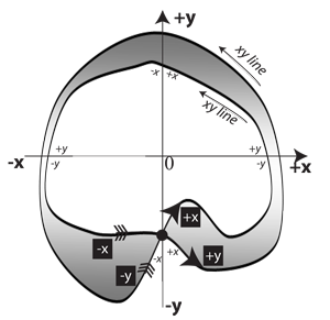
V.1.9 We can easily use our three dimensions to build a Möbius strip. Its surface is then an xy two-manifold that can easily reverse orientations with z. But as in Figure 28, that reversal of orientations is impossible to realize in only two dimensions.
Since that unknot with crossing, complete with indicated area, is a two-dimensional figure, it can only suggest the twisting and nonoriented behaviour we experience so easily in three. It nevertheless helps make our higher-dimensional world’s Möbius twist events at least a little clearer to beings confined to that lower-dimensional one. The definite seeming “interior” regions on both Boy’s surface and our Möbius representation mark them both as “immersions”. Since neither interior reflects the reality, neither is a proper “embedding”.
The Möbius strip we represent in Figure 28 cannot be properly embedded in two-dimensional space. It can only be immersed.
V.1.10 Both Figure 28’s unknot with crossing and Figure 27d’s Boy’s surface make compromises in their efforts to indicate their respective twisting events. The distinction between an immersion and an embedding is that an embedding surrounds any object with all the rest of that space. We have represented Figure 28’s crossing point as a small and filled-in rotagon. It is a large dot fully embedded in that two-dimensional space.
We can similarly surround any three-dimensional object with all the rest of space. But we cannot fully surround four-dimensional objects. We can only immerse—and so indicate—them in our three.
V.1.11 We in our three dimensions can only navigate both sides of a Möbius strip because our extra dimension allows us to twist. Our two-dimensional Möbius strip immersion emulates Boy’s, for a two-dimensional being, by creating a circulating linespace. Since that twisting manoeuvre is not available in only two dimensions, we must resort to self-intersections to represent it. The circulating, unbounded, and noninfinite one-dimensional xy manifold connects the positive x-axis to the negative y-axis, and the positive y-axis to the negative x-axis.
The interior and exterior that Boy’s surface seems to provide is no more real than the apparent space Figure 28’s immersion bounds. When a Möbius strip is realized in three dimensions, there are no such interior or exterior regions.
Boy’s surface tells us where we can find objects in a bigger and higher-dimensional manifold. The four-dimensional space it depicts is at all points tangential to that immersion. Each of these two constructions is only a mapping to each one’s infinitely extended and higher-dimensioned spaces so that Figure 28’s x and y axes truly do go marching off to infinity either side, and do not curve round as the immersion suggests.
V.1.12 In spite of the above caveats concerning its appearances, Boy’s surface clarifies that in order to complete a circulation of the generations, it is necessary to traverse both its sides. Such objects must therefore share the same positive and negative absolute values at all times; across all observable dimensions; and so must also always share the same rates of change and behaviours on their bases, their fibres, their fibre bundles, and their deformation retracts and mapping cylinders.
V.1.13 The symmetries and the rates of change enshrined in our two sets of exact and inexact differentials circulate equally about Boy’s surface. While the three constraints are exact differentials that state the smooth and direct paths common to all spaces, the three stases of the numerical, the material, and the energetic are the potentially irregular surfaces that state the paths leading to, and that can surround, those volumes. They are instead inexact differentials. But since the four dimensions they each represent cannot be properly represented in three, then those planespace rates in x, y and z inform us of the need to master their differences in rates.
V.2.1 Boy’s surface helps us to distinguish between species by demonstrating that the entities in each are constant topological neighbours. They always enjoy each others’ velocities and accelerations. The surface confirms that no matter how far the entities might travel in any given direction, they always end up—still together—at their joint triple point values, so creating their equally curving joint mapping cylinder about themselves. They achieve this by sharing the rates of change that define their joint symmetry or invariance. Those rates over time then become the absolute amounts that distinguish each species. But these are exactly our plessists and our plessemorphs, which always undertake communal transformations. They move between their shared maxima and minima, and so about their common deformation retract, S’ = {n’, m̅’, p̅’}, which they jointly maintain over T.
V.2.2 Each of the three meridians on Boy’s surface is an unknot with crossing constructed from a set of rates. The xy, xz, and yz planes represent the transformations supervised by the constraints, and that are then its surface. Each meridian twists two planes, as two rates, about itself. Each therefore wraps itself about Boy’s surface from one pole to the other, acting as a Möbius strip’s centre line. Each thus forms one of the three biological constraints. Each dimension or manifold interacts with two others to form the meridians that then curl about the entire surface.
V.2.3 The corresponding poles in our biological space are ninitial as the beginning and nfinal as the end of a generation. Those two values define a diametric route, of minimum rate of change, that punches directly across the Boy’s surface interior, creating its triple point, and so defining the overall number density, N. Since those initial and final values incorporate rates, then the greater is the distance, the greater the relative differentials involved.
V.2.4 The equatorial plate in Boy’s surface is now a fourth Möbius strip. It is orthogonal to the above meridional three. It has three twists. It delineates the maxima that the meridians reach as they journey from pole to pole. It defines the fibration–cofibration cum biology–replication globe interface that creates the mapping cylinder for our recursive functions in Figure 7.
V.2.5 The Boy’s surface equator bounds the unit rotachoron. It is a fourth interface between our biology and replication globes. The fibration transforms the other three, which are the meridians, from pole to equator. The cofibration then imposes the reverse transformations to carry them back to the other pole, which is the self-intersection point.
V.2.6 The triple point at the rotachoron’s centre, bounded by the equator, is the deformation retract that the population uses, with the surroundings, to construct a generation. Their complete biological behaviour is the covering mapping cylinder, Mλ, that is Boy’s surface. The surface’s area again states the rates of change. Boy’s surface will therefore help us define a species in terms of a shared invariance or symmetry, in the rates that create the ψ, γ, θ and ρ that is the complete set of biological activities, λ, that construct it.
V.3.1 We then turn to the real projective plane in Figure 27c. Its equator is also an unknot with crossing. It can therefore twist a plane of biological activities about itself. The same goes for its meridian, which contains the crosscap that identifies all diametrically opposite points upon a circle.
V.3.2 Loops upon the real projective plane that do not cross the real projective plane’s equator, and so that do not touch its edges, can only form trivial cycles in one hemisphere or another. Any that touch its edges cross the equator and create a circulation of the generations.
V.3.3 All lines on real projective planes emulate the Boy’s surface equator and its three meridians by being continuous journeys. Both the replications across the biology–replication globe interface and the ingress across the generational interface are continuous journeys. They each have a distinctive length, and a distinctive rate of curvature across all four dimensions. Each loop leaves its initial basepoint, α0. Each then returns to give α0 = F to form a loop, s, in some space, S.
V.3.4 Every circulation of the generations is a continuous loop. But even though every species or biological space, S, can hold a vast array of such loops, s, they will all hold certain characteristics in common.
The common characteristic of all such repetitive journeys is their reversibility. If we go first north then east on any loop s in some space S, we must eventually go south and west or we do not return to the beginning. If a generation is to repeat, then those rates and lengths must cancel out. But granted that these are topological loops, then the distances concerned are potentially unbounded. This unboundedness does not, however, change the essentials of reversibility. Henri Poincaré (1892) first referred to this essential characteristic as the space’s “fundamental group”, π.
V.3.5 As a general principle, each loop s in S remains essentially the same if we instead choose to go about it in the opposite direction. This gives s-1. That reversible succession of rates of change of latitudes and longitudes makes the original, s, and the reverse, s-1, homotopically equivalent. They do the same thing, for they go out and back to the same point over the same terrain, and to the same effect.
Going about the same loop in both the forwards and the backwards directions confirms its smoothness and its path-connectedness. It also multiplies them together, as a group operation, to give s ◦ s-1. This is the “zero point loop” of α0 to α0 or F to F. Since all rates necessarily cancel out, this s ◦ s-1 multiplication is also the “constant loop”.
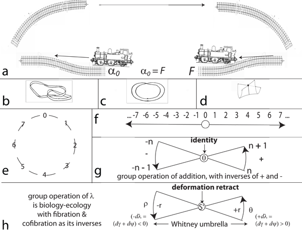
V.3.6 As with all important topological designata, constant loops are independent of size. Figure 29a shows that any two railway lines in a perspective drawing can potentially create a loop. Since they are topological, they can increase any loop’s size by extending, without bound, in any direction. As they move indefinitely far into the distance, the two tracks will look as if they come together to create a single point upon the horizon. That horizon—which represents the unbounded—is the line at infinity. It lies all around as a circle at infinity.
The opposite direction holds the loop’s completion. The same railway tracks approach us from behind, again coming in from a point at infinity. And since they went out to infinity; looped around on the circle at infinity; and then returned as their opposites, again from infinity; then that entire circle out at infinity surrounds us, topologically. It emits and absorbs all such loops. All points upon each such completed loop, irrespective of length and location, are constant topological neighbours. They also indicate rates over lengths that ultimately cancel out, or they would not be loops.
A train can now leave us on its parallel lines; go all the way out to infinity at some initially known rate; circle about while still infinitely far away; and return back from infinity; but over on the other side, and with an opposite rate. The Möbius strip in Figure 29b is now the prototype for all such beginning to end and circulating behaviours (Carter 1993).
V.3.7 A constant topological loop means that we can draw conclusions about any circulation of the generations, and of any size. Each stretch x on any constant loop s in any space X is precisely matched by both (a) an inverse x-1, and (b) a complement, x’.
For each journey x in X, there exists a reverse journey x-1, back across that same interval, and that eventually creates the out-and-back constant loop, s. This is also the identified and opposite points for that expanse, but as if moving in the same direction, over on that opposite side.
The complement of x’ is the remaining span of any constant loop, and such that x ◦ x’ = s. Thus to move along some x in X, and then to turn about and return, is equivalent to having moved all about in that same direction and along some opposite and identified span; and to traverse the entire loop and to return, as if from the opposite direction, and having gone about the whole. To go out a specified distance and turn and return, which is x ◦ x-1, is homotopically equivalent to going about the whole, in the same direction, for x ◦ x’. This gives the equivalences x ◦ x-1 ≈ x ◦ x’ ≈ s.
V.3.8 The Möbius strip is also defined by both its continuous midline and its boundary. The latter is the unknot with crossing of Figure 29c. Its journeyings nevertheless appear to bound the Möbius strip’s area which first diverges steadily from the midline to increase by +dA; and then steadily converges by -dA, leaving a net of zero all about that circulation. The overall absolute value for that area is therefore stated by the amount the midline has travelled. It is a rate that also builds the triple point and deformation retract. An unknot with crossing is thus the prototype for all transformations and rates of change occurring about a central value.
V.3.9 Since a biological population requires Möbius strips and unknots with crossings, then it also demands the Whitney umbrella of Figure 29d. That sends out a line that circles about; returns to the same point; then goes out the other side to do the same. That double loop, s, goes forwards and backwards, once upon each side, giving it its inputs, and outputs, of +r and -r. They are the contacts with both infinity and the surroundings. This is the singular point with continuous neighbourhoods that creates a self-intersecting rectangle on either side.
The Whitney umbrella is now the double point, S0. But it is also our V0 pointspace. It is the symmetric α0 or F zero point that goes nowhere, balancing all lengths and rates simultaneously as S0–V0. Since it can simultaneously emit and receive all forms of opposite behaviours, then the Whitney umbrella is the prototype for all branching behaviours (Carter 1993).
V.3.10 Figure 29e confirms that all these loops s in S are cyclic groups. As with the eight-member group depicted, each element can successively generate the next, under its given operation. At least one is also able to generate all others, including the group’s identity element.
V.3.11 Figure 29f shows that the integers, Z, form an infinite cyclic group. Like all such groups, it is symmetric and has exactly two generators, +1 and -1. Each can generate the entire set. And again as in all such groups, the generators can come symmetrically together to create the identity: +1 - 1 = 0. Every element that is not the identity is of infinite order, for it can generate all the infinitely many others. And for every element, there is an opposite which together produce the identity.
There are infinitely many infinite cyclic subgroups. And since the loops we can create with them can all reach out to infinity and return, then the Whitney umbrella can grow or shrink to any size. Its branch points can create the entire bound that is the equator about any possible Boy’s surface. Every point holds a definite value while still incorporating opposites around a central identity. All Whitney umbrellas can form an infinite cyclic group, plus subgroups and generators, as can generate other infinite cyclic subgroups; and as can also replicate any given population, along with the identity.
Figures 29g and h now show that all biological populations are isomorphic with the field of integers. Whitney’s umbrella in other words has the identical and symmetric group structure as the integers. All biological entities and populations are thus equipollent with the set of countably infinite natural numbers, ℵ0 (Weisstein 2015a). Additionally, no element generated by the infinite cyclic group’s generator is the identity element, but every element that is not the identity is of infinite order, and can generate the identity in conjunction with another.
V.3.12 We now know that to go out on any stretch x along some constant loop s in some space S and then to turn and return is homotopically equivalent to proceeding all about that loop … which is a complete circulation of the generations.
V.4.1 We must now determine what it means to be “in a species” in terms of the fundamental group or groups that all the loops in any space S hold in common, and as distinguish them from all loops in any other space, which means from all other spaces.
V.4.2 Loops 1 to 4 in Figure 27 are in this sense technically equivalent. We can go both forwards and backwards about them all, deforming them into others of that same type. They are all simply connected. They can smoothly contract to the singular point that is their constant loop. Since they are therefore homotopic to that constant loop, they are homeomorphic. These cannot help us separate out species.
V.4.3 Loops 1 to 3, however, are trivial cycles on each of the sphere, torus, and real projective plane. They do not cross any equator. They can help confirm species boundaries.
V.4.4 Loop 4 is different to Loops 1 to 3. It is nontrivial. It crosses an equator. It can help define species boundaries.
V.4.5 The sphere in Figure 27a can host infinitely many loops and cycles, both trivial and nontrivial. If we imagine each loop as a rubber-band, then each can slide easily in any direction. They can all deform freely into each other and into the constant loop. The sphere is therefore simply connected.
V.4.6 All loops upon a sphere have the common characteristic that they can all slide right off. All possible trivial loops for all n-spheres, of whatever dimension, behave the same way. The constant loop is their common identity. A sphere’s fundamental group is therefore trivial. No matter what the dimension, all spheres have the “trivial fundamental group”: π(S) = 0.
V.4.7 Every species similarly has some entities “inside it” by being current and observable. Yet others are “inside it” in the sense of being non-current … but replicatively accessible. They are therefore currently “outside it”; but only in the sense that they have yet to be replicated. They are inside through having the potential to be replicated. They differ from all future entities in all other species which are therefore “doubly outside” by being (a) yet to be reproduced, but also (b) not being inside that species at all by being permanently and replicatively inaccessible. We must find a way to represent this.
V.5.1 Loops 5 and 6 upon Figure 27b’s torus are very different from the loops upon Figure 27a’s sphere. If they were placed back upon the sphere, they would define its equator and prime meridian. But they would also deform and slide off like all others.
When we remove Loops 5 and 6 from the sphere and put them back on the torus, they behave very differently. They have a common contact point upon the toroidal surface. They meet and link. They become impediments to each other. The one on the meridian prevents the one on the equator from sliding off. It is possible to deform the one into the other, so that they switch their directions and their senses of interior and exterior, but they still prevent each other sliding off. These can place boundaries around species.
V.5.2 Every space, X, has a boundary which is the set of points, C, that is its “closure”. It is the subset of its points that can be approached from both its interior and the outside. Any point c in C is a “boundary point”. A “boundary operation” is then that of finding all those boundary points. And even though no noninfinite and unbounded manifold can be built in the same dimension exhibited by its local topology, boundary operations determine their characteristics by studying them at the level of both (a) the two-dimensional plane; and (b) the one-dimensional line.
An interior point can move freely in all relevant directions, unrestricted by any closure or boundary. A two-dimensional plane’s interior is any space homeomorphic to a disc or rectangle. Each interior point is then surrounded, on all sides, by others. Thus a sphere’s surface—considered independently of its interior—is again homeomorphic to an infinitely extended plane. We do not find a boundary point in any direction.
The same holds for a line. An interior point in one dimension is surrounded by others. So no matter how far we might travel along a circle, we find no boundary point. There are always points to either side. Thus a circle is homeomorphic to an infinitely long Euclidean line.
If we now imagine a disc or rectangle cut in half, then its boundary points only surround a half-plane. The boundary point now has an interior point on one side, and an exterior one on the other. A half-plane is not homeomorphic to a full disc. This holds true whether we stretch or shrink it.
The boundary we have just discovered is instead homeomorphic with an arc that has endpoints on either side. If we stand at the arc’s midpoint, then any journey out to one end point is the same as a journey to the other. We get to a boundary point either way. So we can just as well close up the arc and draw those two end points together. We now have a line segment. And since that line segment has the boundary point at its end and no points beyond, then an arc is homeomorphic with a line segment. The half-plane in its turn consists of all points on one side of an infinite straight line, and no points on the other. We can thus use either the half-plane or the line segment to separate any space.
V.5.3 We can define these anomalous interiors and exteriors for our biological populations by considering the fundamental polygons belonging to the sphere, the torus, and the real projective plane, and then undertaking their respective one- and two-dimensional boundary operations. We first take up the torus in Figure 27b.
V.5.4 The torus’ fundamental polygon is a full plane. Its edges can be freely pushed to either plus or minus infinity. Boundary points advance and retreat as we approach, without us ever walking into them. Since we can create any torus, of any size, simply by gluing the ends of any cylinder or its fundamental polygon together so the arrows align, then just like a sphere’s surface, a torus’ would appear to be homeomorphic to an infinite Euclidean plane. There are always more points in the interior, acting as a full plane and rectangle. We again do not find boundary points.
V.5.5 We can then perform our one-dimensional boundary operations, on the same torus, by applying a retract hyperplane. It becomes an annulus in the plane. And if we next deformation retract those two edges by drawing them inwards equally, the annulus eventually becomes a circle and a one-manifold. We can walk about that circle infinitely in every direction, without ever finding a boundary point. Since this is also equivalent to an infinitely long line, then the torus has no points in any C or closure set. It therefore has c = 0.
V.5.6 A sphere is unfortunately very different.
V.5.7 We already know that if we cut a sphere in half and then flatten it out into two dimensions, the hemisphere’s edge goes all the way out to infinity, and we get a real projective plane. The sphere’s fundamental polygon, in Figure 27a, is therefore very different from the torus’. It might look like a full rectangle … but it is not. It is instead two of our half-planes abutting, each separately bounded by an infinite line.
If we glue the edges of the sphere’s fundamental polygon together, the surface becomes infinite and unbounded. It is homeomorphic with an infinitely extended plane. However, the sphere itself is a three-dimensional object. And … that has an interior and a bound. It will always have that interior. If we try contracting it to a point, we will always find a set of interior points, with a boundary sitting right beside them. Despite its surface having the local topology of a Euclidean plane and always being unbounded, the sphere’s interior always has a point of closure, or an edge.
Walking along the boundary of the sphere’s fundamental polygon produces a further problem. Since identified points go in opposite directions, from the same point, then we cannot get to the other half-plane without crossing the hemisphere’s boundary … which is an edge. If we measure the flattened hemisphere using spherical coordinates, the plane goes out to infinity; and we return upside down on the other side. If we want to replicate those opposite behaviours then we must remove a line from the full plane to create two half-planes; or we must remove a point from a line to create two line segments, This is equivalent to saying that the boundary point always exists.
We can express the above by saying that the sphere is a bidimensional manifold with an infinite plane for each hemisphere. Each set of points in each of its half-planes has a neighbourhood homeomorphic with the neighbourhood of a point that belongs to the closed half-plane’s boundary or closure set, C. Each half-plane is an arc containing a boundary point, c. The sphere is a line with central point removed to create two line segments, and therefore has c = 1.
V.5.8 While it is true that the torus’s surface can emulate the sphere’s and support a complete set of infinitely many rubber bands equivalent to the sphere's π(S) = 0 trivial cycles … the ones we place on a torus’ meridian or equator have an important restriction. Those two sets—such as Loops 5 and 6—are very different from all those we can place either on a sphere, or elsewhere on the torus’ surface.
The torus has a double interior. There is the volume that creates its “filling” when it is a doughnut; and there is the volume behind the surface that makes up its doughnut body. Since the torus has that hole in its middle, none of the infinitely many rubber bands we can place about its prime meridian can slide off. But further since its surface is infinitesimally thin, all rubber bands placed about the prime meridian automatically conjoin with any placed about the equator. And since one set is born from an annulus—which has no closures—then none that bound either the prime meridian or the equator can contract to a point. Each is held fast by the other.
We now find that the only rubber bands that can slide off a torus are its trivial cycles, similar to a sphere. Those, however, bound neither its equator nor its prime meridian.
V.5.9 The torus now differs significantly from the sphere because the two sets of infinitely many non-contractible loops we can place about either of its two diameters are each independently equipollent with the integers, Z. And since none of the three sets of loops the torus has available to it can be persuaded to slide off by first deforming them into any of the others—for two sets are linked—then the torus’ fundamental group is very different from the sphere’s. It also guarantees us both an equator and a prime meridian for our nontrivial biological loops. It has π(S) = Z2.
V.5.10 We now have both an equator and a prime meridian. This is both (a) a beginning and an ending for our biological circulation, plus (b) a maximum and a minimum. But the two are linked. We cannot yet separate them from each other. We still cannot distinguish the biology–replication globe interface from the generational one that marks the beginnings and ends of the circulations of the generations … although we must travel to them all.
V.6.1 We now look at the real projective plane’s Loop 7, in Figure 27c. This is ostensibly the same as both the sphere’s Loop 4, and the torus’s Loop 5. Those each go about their respective equators. But the projective plane is like the torus in being an infinitely extendable plane with no boundary points: c = 0. However, since Loop 7 is only a loop because its opposite points have been identified, then it is not a loop upon its particular surface. It is a line segment. The projective plane therefore has a different fundamental group from both the sphere and the torus.
V.6.2 None of the loops located inside the real projective plane’s fundamental polygon, in Figure 27c, touch its boundary. Like all the π(S) = 0 ones on the sphere, they are all contractible trivial cycles.
However, Region 8 on the real projective plane is highly deceptive. The plane’s two parts might look divided, but all its regions—including these abutting the boundary in that Region 8—are locally Euclidean. Since they are identified, we jump smoothly from one point in a Region 8, on one side, to exactly that same point on the opposite side. But as the equivalent Regions 8 upon the sphere and the torus in Figures 27a and b suggest, we teleport across an entire hemisphere to get there.
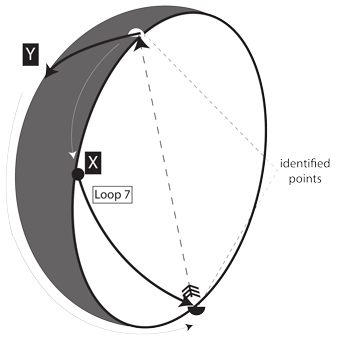
V.6.3 Figure 30 clarifies what is happening. Loop 7 begins in hemisphere X on the real projective plane, which travels on the sphere’s inside. When we hit the equator and boundary—which identifies opposite points—we immediately teleport to the equivalent point diametrically over on the opposite side. We have only physically crossed the equator once.
We now travel in the same direction, in hemisphere Y. But this is on the sphere’s outside.
When we arrive at the equivalent and identified point opposite our Loop 7 start, we are therefore over on the opposite side, in Y. But since there are many points in X we teleported over and have not traversed, we have not yet completed a circulation.
We must now keep going in the same direction. We must travel right across the projective plane and return to the equator to teleport a second time. That second teleport takes us to the same point at the top. We can then travel upon the inside to go back to the start of Loop 7 in X. Only now do we pass through the same identified points we just covered in Y, so we can complete the nontrivial loop, s.
Figure 30 makes clear that we must in fact travel through some Region 8 twice to circumnavigate a globe. This is equivalent to saying that if we begin at some initial α0 and go forwards to hit some maximum; and if we decrease from that maximim to return to α0; then we have only completed half a circulation. We have travelled about only one loop on a Whitney umbrella. We must keep going past α0 to some minimum and then reverse to re-approach α0 from the same side. We then complete the loop, s in S, with the return to α0 being the final point, F.
V.6.4 If a first line representing some journey upon a real projective plane goes to the edge and then reappears from the opposite boundary, but in the opposite hemisphere, then a second line must eventually go back to the original hemisphere, to complete the journey. And if we deform a first loop along one boundary so it moves smoothly into a nearby region at some given rate, then we must deform its complement equivalently smoothly upon the other boundary, at that same given rate. We must always consider all lines twice: once for each opposite hemisphere.
As in Figure 27c, a complete journey across a real projective plane always has two complementary line segments symmetrically placed about a middle one. A completed journey is effectively two complete lines. And since we have to loop twice about any such curve to complete a circulation, then the real projective plane’s fundamental group is a cyclic group of order two: π(S) = Z2.
V.6.5 A cyclic group—even if only of order 2—always requires that some subgroup contain a member that can generate the whole. As with all other cyclic groups, this latest Z2 one must have the identity, #, for its first element. The other must then be the sole group member.
Let the sole member in this cyclic group of order 2 be x. Since it is the only member in its cyclic subgroup, then we take it up and add it to itself. This steps us through to the next group member. But that must be the identity. There is no other possibility. This gives x ◦ x = #. And since the only two group members are x and #, then x has suitably generated the entire group. We thus have <x> = {x, #}.
V.6.6 If we now take up the identity and add it to itself, we do not step to the next group member. We instead get # ◦ # = #. Adding x to the identity also keeps it invariant, as in # ◦ x = x ◦ # = x. Since the identity never generates x, we have <#> = {#}. This cyclic group of order 2 therefore has both the entire group and its sole member for its cyclic subgroups.
This cyclic group of order 2 is immediately homeomorphic with the two line segments in Figures 29g and h. They abut each other to give opposite and infinite loops upon either side. The two together are now a line with point removed from between them. That removed point is their identity, for it acts the same to each, being their respective boundary points. They are each now a half-plane and an arc, the whole creating a sphere. And since each of those line segments can also be a constant loop, then we have our Whitney umbrella.
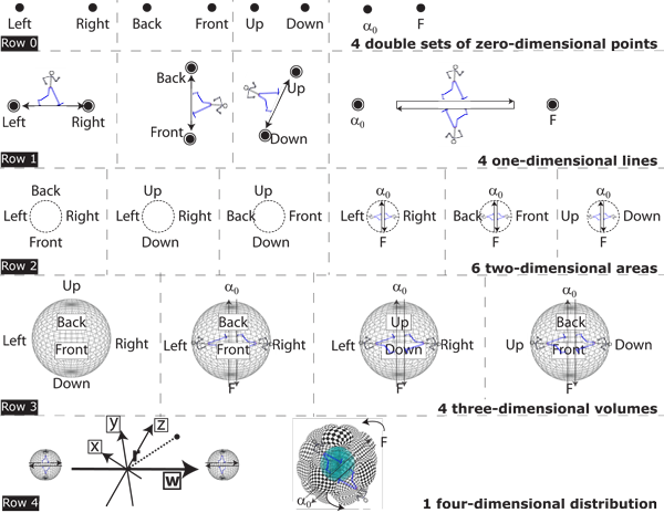
V.7.2 While it remains impossible to represent four dimensions in only two, Figure 31 demonstrates that since biological entities and populations are communities of rates, then they are infinite cyclic groups constructed from four of Figure 29h’s Whitney umbrellas.
V.7.3 Row 0 in Figure 31 is the complete set of four pairs of zero dimensional points. They are the S0 0-spheres that establish our four-dimensional rotachoron.
The four S0 points are also point-pairs. Those point-pairs—±x, ±y, ±z, ±w—create our V0 pointspaces. But when placed in a Euclidean situation, those opposites coalesce and act singly, presenting as |x|, |y|, |z|, |w|. They are coincident, establishing a common S0 value.
V.7.4 Row 1 pushes the coincident ±x, ±y, ±z, ±w pairs of 0-spheres apart, as a step-up, to create the one-manifolds that can hold our lines and linespaces. They are the 1-balls that state the distance between the 0-spheres they have at their ends. They are then separated by the distance 2r. Since ordinary physical space is much more familiar, we temporarily label the first three sets Left–Right, Back–Front and Up–Down. The fourth pairing of α0–F establishes the beginning and endpoints for a constant loop. These all give the equivalent of ∇Q = 0 as their gradients. And since the distances between them can vary while the gradient remains the same, then they are again inexact differentials.
V.7.5 Row 2 brings our various 1-balls together, in pairs, to create the various step-ups that are our (x, y) 2-ball planes and planespaces. Each 2-ball is bounded by its 1-sphere, which is a one-manifold. But each also has a 1-ball stretching diametrically across its middle linking that 1-sphere to that 2-ball area. The diametric 1-ball directly linking the relevant identified 0-sphere points can thus tell us how either the 2-ball area, or the bounding 1-sphere line, is changing. The generation’s beginning can, for example, shift its position at some given rate, relative to its ending. The 1-ball therefore measures the divergence created by the 2-ball. These together give ∇ • Q = 0. This is also an inexact differential, for the amounts can change while the divergence remains the same.
V.7.6 Row 3 brings the six 2-balls together to create the various (x, y, z) realms and realmspaces. Each 3-ball is bounded by a 2-sphere which is an unbounded but non-infinite manifold. Both the journey along the 1-ball diameter, and that about the surrounding 2-sphere can tell us how the contained volume grows and/or changes relative to each. So if our 3-ball contains α0–F then we again know how rapidly properties change across the generation. We know how rapidly the volume is changing due to the gradient and divergence. These together give ∇ × Q = 0. And since the quantities can again change while the curl remains the same, then these are yet more inexact differentials.
V.7.7 And then for Row 4, we take a yet further step up, or integral. If we take up any of the rotahedrons in Row 3 and push them out along the remaining dimension, we will create the identical (x, y, z, w) rotachoron each time.
We can understand this last step-up as a distribution. We can, for example, consider inflating a hot air balloon; or else measuring the atmosphere, with its different densities, at different heights. We can draw a graph of all the balloon’s different volumes at each point in time as we inflate it; or we can record the atmosphere’s density per unit volume at a host of different heights. We will then have the balloon’s rate of change in its volume across the entire interval; or the rate at which the atmosphere’s density changes, in each volume element, at all points. We can now compute how much air the balloon holds at each point, as well as the total moved in and out; or the atmosphere’s mass. We in each case know a given property’s distribution across some fourth dimension. In the same way a four-dimensional Lorentzian spacetime tells us how gravity is distributed.
Our fourth biological dimension is now telling us how different biological populations distribute their various activities both across an elapsed absolute clock time, T, and their generation length, τ.
V.7.8 Biological populations also combine their numerical, material, and energetic stases to give ∇Q = ∇ • Q = ∇ × Q = 0. And since these are all inexact differentials, then the size of the rotachoron they form can change even as these stases of the first, second, and third kinds remain identical. A circle, for example, maintains certain properties as invariant, even if the actual sizes of radius, area, and circumference all change.
V.8.1 We have a set of both exact and inexact differentials in ∇Q = ∇ • Q = ∇ × Q = 0 and ∫dn = ∫dM = ∫dP = 0. We are looking to equate them in some group operation, ◦, that we can perform on some biological population. That group operation should also leave some x or y in the group essentially the same. We will then have our strictly biological identity property, #. Since it is indifferent to both exact and inexact differentials, then we will be able to relate the two sets through that identity.
V.8.2 All events in both our biology and replication globes affect the surroundings. They are therefore temporal. As in Figures 32b and c, the biological events that create a circulation must therefore have some temporal ordering with respect to each other.
V.8.3 But as in Figures 32a and c, we can also analyse those same events from a strictly biological perspective. We can assign those same events to one or another of our biology and replication globes based entirely on their effects. Since similar biological events can occur at different points in the cycle, those effects are irrespective of that temporal ordering.
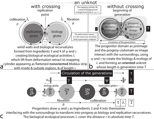
V.8.4 Figure 32a is two-dimensional. It has a clear but doubled up interior contained inside the unknot with crossing. Figure 32b is three-dimensional. It appears to be the volume defined by a Möbius strip’s twisting loops. But since it is embedded, there is no demarcated interior or exterior:
• The two discs in Figures 32a use the replication point—which is their identity—to create a Whitney umbrella of pointspace, V0. They also present themselves as the singular point S0 of specified properties. The total recurvature distance about the two discs—and also about Boy’s surface—is τ.
• The two globes in Figure 32b arrange the same events temporally. Their diametric distance is the absolute time span, T, for the same events. That distance punches across Boy’s surface. It passes through the triple point at its centre.
• Figure 32c combines both the above as the dt = Tdτ of biological-ecological processing, λ, that completes a generation. It represents the minimum criteria any population must satisfy to create a fibration and cofibration, and to class as biological.
V.8.5 We have equivalent ways of understanding biological events. Each of the biology and replication globes recurves—i.e. distributes—its ingested materials about itself, building and/or maintaining its wind walls. Those are its ongoing biological activities, λ. They must also be observable and temporal. Their configurations are the volume and semantics, V. They have the surfaces and syntax, S:
• All replicative materials must be biological, but materials can be biological without being replicative.
• All biological events begin, temporally, at some identified point, or equator, and then distribute themselves across time, but none are obliged to complete such a cycle and reach the end of any generation.
• While everything homeomorphic is both homomorphic and homotopically equivalent, not everything homomorphic and homotopically equivalent is homeomorphic.
V.8.6 We begin a recurvature in Figure 32a about the two-dimensional discs and doubled-up interior at their contact point, which is also the replication point. The fibration, θ, carries us anti-clockwise about our biology disc, simultaneously lifting us from deformation retract to mapping cylinder.
When we return to the replication point in Figure 32a, we have only travelled half-way about the Möbius strip. We have inverted some value from +r to -r, or conversely. Since we are currently going in a direction opposite to the one we first started with, we must keep going to complete the cycle.
We next enter the replication disc. We undertake the cofibration, ρ. We eventually get back to the replication point. We are back to moving in the original direction. We have travelled completely about the doubled-up interior, and used our Whitney umbrella and Hooke cell to fully restore S0–V0. Since everything is now the same, we have found our biological ◦ operation. It is this journey around both globes.
Any of our plessists and plessemorphs that go around this Möbius strip and complete a circulation of the generations must abide by:
• Closure, because if x and y are each along that path, which is to be in the group, then x ◦ y is also in the group.
• Identity, because there is an #—which is the journey that passes twice through the replication point before returning to some original point in the same direction—and such that for any x, going all about both globes gives x ◦ # = # ◦ x = x. And since τ is the time required for that generational identity operation, then x ◦ τ = τ ◦ x = x. We have τ = #. There is a definite amount we can change by that leaves all the same.
• Inverses, because for any distance x, there is a complement distance, x’, that completes the recurvature, and so that x ◦ x’ = τ and x’ ◦ x = τ. But there is also the distance x-1 that creates a constant loop, and so that x ◦ x-1 = x-1 ◦ x = #. This inverse and the complement together produce x-1 ◦ x’ = x’ ◦ x-1 = |τ|, with the inverse being the shorter of these two distances. It creates the opposite effect to x, so that applying it to x is the same as moving about the whole, as in x ◦ x-1 = x-1 ◦ x = x ◦ x’ = x’ ◦ x = τ.
• Associativity, because if x, y and z are in the group then (x ◦ y) ◦ z = x ◦ (y ◦ z).
V.8.7 Figures 32a and b represent the two interconnected ways of understanding the cycle of the generations. The former is τ and nontemporal and nonoriented; the latter is T and temporal and oriented:
• Figure 32a is concerned solely with τ and globe allocations. The biology and fertility globes balance their λ biological activities by distributing their γ and ψ Ingredient 3 and 4 events between themselves. But since they ignore temporality, they are nonoriented. The biology globe is entirely nonreplicative. The replication one handles all such events. They together provide our interior recursive functions. The sum of the curls about each is the stasis of the third kind, ∇ × Q = 0, and is the circulation of the generations.
• Figure 32b is concerned solely with arranging events in a temporal sequence, T. While it can distinguish between increases and decreases in γ and ψ, it makes its temporal markers take priority over any proposed distinctions between the biological and the replicative. They each predominate in distinct epochs. The γ increase phase, which is m and Ingredient 4, has a smaller range than the similar ψ increase phase, which is p and Ingredient 3. There will therefore be times when the latter increases while the former is stationary, or even reverses. Since these events are successive, they are oriented. Their ordered activities provide our loops. The sum of the divergences is the stasis of the second kind, ∇ • Q = 0, and is once again the circulation of the generations.
• Figure 32c represents the sum of the events in both globes, and is ∇Q = 0 and the stasis of the first kind.
These inexact differentials are independent of size in the sense that they can produce the same, overall, effects, of leaving everything the same, but over greater and smaller ranges. While they may have apparently different effects out in the surroundings, their overall purposes on the objects are the same.
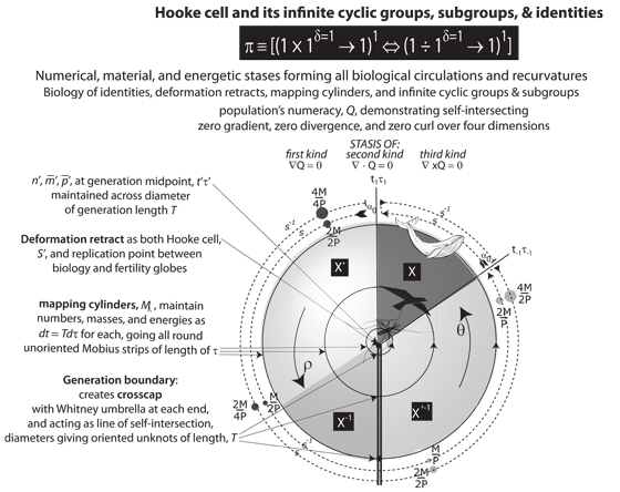
V.9.1 We now turn to the representation of Meme 112 we see in Figure 33. It sets the three constraints and exact differentials of ∫dn = ∫dM = ∫dP = 0 equal to the three inexact differentials and stases of ∇Q = ∇ • Q = ∇ × Q = 0 using a set of group operations. It is the four-dimensional S3–V4 rotachoron. It is the regular V4 gongyl or interior, surrounded by its four S3 glomes as its combination and surface. It holds an entire collection of the constant loops that we can build, at any time, using its plessists and plessemorphs. They display the combined exact and inexact equilibria. They also immediately give us the π(S) = 0, π(S) = Z2, and π(S) = Z2 fundamental groups for all trivial loops, equators, and identified traversals between minima and maxima.
V.9.2 Meme 119 now declares that each of the τt, τn, τm, and τp one-manifold linespaces that create Figure 33’s balanced rotachoron has its opposite points identified. Each is a spherinder contained within a cubinder. Each is therefore a diameter. Each supports an entire equator of surfaces and activities for Meme 3’s unipollent equilibrium of π ≡ [(1 × 1δ=1 → 1)1 ⇔ (1 ÷ 1δ=1 → 1)1].
V.9.3 We also follow Euler, so that for Meme 120 we express all increments in Figure 33, over all populations and generations, proportionately. We use e and a unit interval. Each increment is therefore a function of a suitable identity process starting at unity and growing continuously and exponentially for one unit. Every infinitesimal increment dx, at all points, is some proportion of the x at that instant. And since all measures are taken between 0 to 1, then they are all expressed in identical units. So if some interval for the insect on the inside is x% of its overall generation length, then the bird and whale outside it exhibit the same proportion. And if some given interval allows some insect, on the inside, to double in whatever property, then the bird and whale outside it will also double, across corresponding intervals.This is a unit rotachoron.
V.9.4 The τn, τm, and τp one-manifolds from Figure 19 meet at the triple point at the rotachoron’s centre of τt’. It has a single point as its V interior, surrounded by its closure points. Those use a Whitney umbrella to form a continuous circle that is the surface all about it.
V.9.5 There are matching line segments everywhere between diametrically opposite—and so identified—points. Since all the one-dimensional braid-1s are coordinated in Figure 29h’s Whitney umbrella, the τ circulation in Figure 33 always passes exactly twice through Figure 32’s replication points to give x ◦ τ = τ ◦ x = x for all x in X. We can create a constant loop at every point in our unit rotachoron.
V.9.6 The implication of x ◦ τ = τ ◦ x = x for all x in X, in our unit rotachoron, is that the centre point is the deformation retract. The surface is the mapping cylinder, complete with all its bounding π = [(1 × 1δ=1 → 1)1 ⇔ (1 ÷ 1δ=1 → 1)1] intervals. Those intervals create the constant loops at every point.
V.9.7 The further implication of our unit rotahedron is that each and every entity and population throughout X is immersed in a universe in which it can use the two S0 input and output points on its Whitney umbrella to maintain itself. The biological–ecological λ is the group operation, ◦. Its positive and negative aspects are the fibration, θ, and cofibration, ρ, respectively, to give θ ◦ ρ = # = λ.
V.9.8 The topological reality is that every population’s biological space is locally isotropic. Since the surface stretches from 0 to 1 for all populations and entities; and since all values and rates are proportionate and dependent upon quantities present; then all plessists and plessemorphs everywhere are the same. They all see the same universe in which they can all sustain themselves. Since all entities and populations receive exactly what they require, at every point, to undertake all needed interactions, then every population’s biological universe is also always locally homogenous.
V.9.9 Since every biological population lies upon some Figure 33 surface, then every point about any viable circulation is in principle capable of constructing a constant loop, for a complete circulation, which always has its opposite points identified. Our S3–V4 biological rotachoron also therefore allows populations to loop between minima and maxima and complete a circulation. We can create the complementary constant loops all about the rotachoron.
V.9.10 Every population and species is locally defined by this identical rotachoron, which states all global realities. The resulting cycle and its loops will satisfy both our defined π equilibrium for our plessists and plessemorphs and their exact and inexact differentials, and the Chomsky production rule of [Σ, S, δ, α0, F].
V.10.1 We can use Figure 33 to consider some Subpopulation X. Its initial point is α0X. Its initial circulation point and time is τ-1t-1. It increments the distance dτX–dtX to reach τ1t1. There is a proportionate effects on all subpopulations. They form the same constant loop, sXsX-1.
V.10.2 Each constant loop for any Subpopulation X is precisely matched by two others. One is the complement X’, the other the inverse X-1.
V.10.3 There exists a reverse journey, x-1, for every journey x in X. It moves across that same interval to create the constant loop, s-1. It implies that every population will return every atom and molecule removed back to the surroundings, thus restoring itself to its prior condition.
V.10.4 We can therefore always form the inverse subpopulation X-1. It also has a constant loop formed via the underlying real projective plane’s identified points.
V.10.5 We get X-1’s initial and final points from X’s final and initial ones, respectively. It is therefore located diametrically across the rotachoron, linking via the central point, which is the deformation retract.
Subpopulation X-1 exhibits a cofibration for every fibration in X and conversely. Its constant loop sX-1sX-1-1 is now the precise inverse of X’s.
V.10.6 The X and X-1 populations are inverse couplings. They sit opposite each other on the rotachoron. They therefore form a cyclic group of order 2.
V.10.7 Subpopulations X and X-1 immediately confirm our π(S) = Z2 fundamental group. Each of the two line segment pairings, on the two margins, creates a set of half-planes that define our sphere’s interior. They are each also a Whitney umbrella whose diameter has the two constant loops that confirm both T and the +r and -r inputs and behaviours. The identity, as the deformation retract, sits between them. Their joint interactions define the surrounding mapping cylinder, Mλ.
V.10.8 We can also form the complement Subpopulation X’. This has X’s terminal point, τ1t1, for its own initial point as α0X’.
We then increment X’ all about the remainder of the circulation until we reach X’s initial point, τ-1t-1, which becomes X’’s terminal one. That complement journey also restores that same population to its prior condition, returning every atom and molecule to the surroundings. Subpopulation X’ thus forms the constant loop sX’sX’-1 all about that remaining circulation.
V.10.9 Our complement X and X’ coupling, that goes all about the rotachoron, contains two sets of inverses. It incorporates the X-1 inverse in its middle, as the inverse to X. But it also has X’’-1, for its last part, and as the inverse to the first part of X’. Therefore, when we add the entirety of the X’ complement to X, we get loops all about the circulation of length τ. They create π. They again define both the deformation retract and the surrounding mapping cylinder.
V.10.10 Going all about the Figure 33 circulation in a forwards, or anticlockwise, direction, is exactly the same as going about it in the backwards, or clockwise, direction. We get the identical constant loops. They both invoke (a) the direct series of biological processes, λ, which map directly between X and Y; and (b) a whole series of inverses and complements, the whole of which always map to Mλ.
V.10.11 Every interval can bring together its XX-1 and XX’ couplings to create both (1 × 1δ=1 → 1)1 and (1 ÷ 1δ=1 → 1)1. But any population that achieves this does so using both of its exact and inexact differentials.
V.11.1 Our exact and inexact differentials may be theoretically equivalent, but Euler established topology by demonstrating that all the points forming any of the Knigsberg landmasses can be collapsed down to a single one; that all the bridges form simple lines as edges which can be deformed; and that all regions can adopt any arbitrary size or shape. They are topologically equivalent throughout because their Euler characteristics, χ, maintain a continuous mapping that preserves their deformation retract. If X and Y are two such sets, then they have identity properties such that an i0(X) exists in X that acts as #, mapping directly onto its equivalent # in Y, which is i0(Y) in Y. This gives χ(X) = χ(Y). We then have Y being a deformation retract for X, with an x in X for every y in Y.
V.11.2 Our Xs and Ys, however, are biological. Since they must each both replicate and be replicated, then they are each both the causes and the products of such cycles.
V.11.3 Since X is the progenitor domain and preimage, while Y is the progeny codomain and image; and since we want to produce a next generation; then we require a reversibility. Since Y must in its turn become an X and act as a progenitor domain and preimage to some further set Y which is then its progeny codomain and image, and with each of X and Y behaving identically and successively … then we require a reverse mapping between X and Y. Every point y in Y must be able to substitute itself back into X and restore X to its original condition.
V.11.4 We therefore require that an i0(Y) in Y exists that acts as #; and that an i0(X) in X does the same; with each mapping directly to give a χ(Y) = χ(X) to match the above χ(X) = χ(Y), there then being a y in Y for every x in X; and with X now being the deformation retract for Y.
V.11.5 We are demanding that both X and Y maintain the identical π equilibrium, with the identical forwards and backwards mappings. They must each have a (1 × 1δ=1 → 1)1 across their lengths for the other’s (1 ÷ 1δ=1 → 1)1; and conversely. Since their forwards and backwards directions must be identical then all mappings between them are only ever both (a) one to one, and (b) onto. They must be continuous bijections.
V.11.6 We are further demanding that both of X and Y be equally endowed with both of our exact and inexact differentials.
V.11.7 Both of X and Y can form fibre bundles. We are therefore and effectively demanding that they each remain reversibly homeomorphic throughout all possible transformations as each is first base, B, and then fibre, F, creating their joint and invariant product space, P = B × F … which must also be their mapping cylinder, Mλ, so that Mλ = B × F.
V.11.8 We are now making the topological demand that every neighbourhood in P look exactly like the composition B × F … and that it never look any different. This is the demand that if one is a set of exact differentials then so is the other; and similarly for the inexact differentials. But since the mapping cylinder is the surroundings, then this is the requirement that each of X and Y fails to act, by turns, as progenitor and progeny when the other seeks to act as a complement.
V.11.9 Although our rotachoron from Figure 33 has given us both an interior, V, and a surface, S, that can support our various biological activities, it is a bidimensional manifold. It is an object whose two halves are separated by an infinite plane.
V.11.10 (A) The rotachoron’s π(S) = 0 fundamental group seems to guarantee all our trivial loops. (B) The real projective plane’s π(S) = Z2 seems to guarantee us all our nontrivial loops. (C) The torus’ π(S) = Z2 fundamental group seems to guarantee us both a meridian and an equator.
V.11.11 The torus is certainly helpful, but it unfortunately has that doubled-up interior.
V.11.12 We can create all the fibre bundles we need by walking a fibre around a base. We can create a base by beginning with an ordinary one-dimensional Euclidean line segment. We then bend it around to create a circle … which is the same circle we get by first flattening a torus into an annulus; and then retracting it. We create a “one-torus”.
V.11.13 We create our one-torus by looping an original line segment around. We enclose an interior area. We therefore began with an object of dimensionality n = 1, and then not only did we separate an interior area from an exterior one, but we stepped up a dimension to get the n = 2 circle.
V.11.14 We can create an ordinary three-dimensional torus from its fundamental polygon of Figure 27b. It has the dimensionality n = 2. We then perform those two gluings. The first gluing steps us up a dimension to n = 3 to create a cylinder, which has a volume interior and those open ends. The second gluing bends that cylinder around to seal those open ends to create our torus.
V.11.15 We may now have our two-dimensional surface all about that torus, but we stepped up a dimension to get it. We also enclosed the torus’ two distinct volumes. We have that doughnut hole in the middle acting a first interior. And we have everything behind its surface, and in its loop, forming a second interior. A torus is therefore an object whose n-dimensional surface always exists in n + 1 dimensions.
V.11.16 And … we have our four-dimensional S3–V4 rotachoron.
V.12.1 Figure 32 took our X and Y progenitor domain and progeny codomains to give two ways to represent our circulation of the generations. Figure 32a’s two-dimensional unknot with crossing flattened our biology and replication globes into two discs. Just as with the torus, we have a clear exterior, but a doubled up interior. Figure 32b was a three-dimensional figure that conjoined our two globes at a single contact point. But since it is bounded by a Möbius strip, its biological events also have no true interior or exterior. It confirms that all Möbius events involve a doubled up interior.
This simply means that any population produced by acts of fertilization and germination must itself create some fertilization and germination events. It therefore approaches the same sizes and activities from the opposite direction, and about the same loop for an s ◦ s-1 = τ. And further since we keep switching directions, then these are nonoriented objects.
V.12.2 The French mathematician Camille Jordan was the first to fully investigate these issues of what properly separates an interior from an exterior. A trivial curve, on any planar surface, is the most obvious of all “Jordan curves”. These are curves, in the plane, that successfully separate a single and continuous exterior region from a single and continuous interior one.
V.12.3 A Jordan curve is the model for going around either the inside or the outside of something, without changing orientations or crossing over to any other side. Anything that abides by a Jordan curve, and so that can successfully separate a single and continuous exterior region from a single and continuous interior one, has an orientation given by ε = 1. Both a sphere and a torus therefore have that orientation.
V.12.4 If we now draw a properly oriented and trivial Jordan curve, as a loop, upon a sphere’s equally oriented surface, we can snip that curve out. We remove a disc from the sphere and make a hole. The remainder of the sphere is homeomorphic to an ordinary Euclidean plane.
If we first deformation retract our Jordan curve, or trivial loop, right down to a single point before using it to snip, the remaining planespace is still homeomorphic to a disc. When the German mathematician Bernhard Riemann first studied surfaces more closely, he described them in terms of such simple and closed curves, pointing out that this was a characteristic invariant for every surface. When Alfred Clebsch later studied this phenomenon, he used the term genus, g, to describe it (Hirzebruch & Kreck 2009).
The sphere is a compact and oriented surface, S, that can support a maximum of zero non-intersecting and closed Jordan curves before it becomes disconnected. It has both an orientation of ε = 1, and a genus of g = 0.
V.12.5 The torus—which can guarantee us our equator—behaves very differently under these Jordan curves. If we apply one to either its equator or its prime meridian, it maintains its ε = 1 orientation, but splits in two to revert to a cylinder. It therefore only takes the one cut to disconnect this manifold.
If we now apply a second Jordan curve to that resulting cylinder, we get a plane surface. We indeed arrive back at the torus’ fundamental polygon, for we can draw on it yet more proper Jordan curves.
If we now reverse our snipping procedure and begin from the torus’ fundamental polygon, we can glue it twice to recreate the torus. Its genus is therefore reckoned either as half those snippings and/or gluings; or else as the single cut that disconnects it. So while a torus has the same ε = 1 orientation as the sphere, since it can support one cut and still not become completely disconnected, then it has the very different genus of g = 1.
V.12.6 Nonoriented objects, with their doubled up interiors, behave somewhat differently under these Jordan curve snippings. While we have a single exterior, we have those doubled up interiors. One part is located either side of the crossing point. And since we can keep switching orientations and directions every time we pass through at least one given point, then an unknot with crossing, such as Figure 32a, fails to be a Jordan curve. Such doubled up and nonoriented objects, which keep switching, have an orientation given by ε = 0.
V.12.7 We can now take up each of our biology and replication globes. If we remove a single point from each, they each flatten to become simple two-dimensional discs. We can then attach them, at their singularities, to create Figure 32a’s Whitney umbrella. We have recreated that doubled up interior bounded by a nonoriented ε = 0 unknot with crossing.
V.12.8 We can now take up those conjoined discs and separate them by snipping, at that crossing, with a single cut. The two previously separated interiors are linked. We finish off with an object homeomorphic to a disc that has a distinct interior and exterior. We have a simple closed curve in the plane that abides by Jordan’s theorem.
V.12.9 We now go up a dimension. We begin with two of our oriented rotachorons. We take one biological and one replicative one. If we next remove a point from each, then they each become homeomorphic to a three-dimensional realmspace. And if we connect them at their singular points, then we have recreated Figure 32b. We have a clear exterior, but the same doubled up interior bounded by a Möbius strip.
V.12.10 If we snip our creation at its crossing, the interiors will link up to give a single interior, and a single exterior. It gives us a realmspace. We have an object homoemorphic with a sphere.
V.12.11 However, if we now set out from a pole, on our creation, and head towards the opposite pole, the crossing point on the original has morphed into an equator. We have gone all the way about a loop, or globe, to the crossing … now masquerading as an equator. We reach the Whitney umbrella branch point. If we continue on, we will branch to the other loop. This is to go past the equator, and to traverse the opposite loop or globe.
V.12.12 A complete twisted journey about a nonoriented ε = 0 Möbius strip type object is now homeomorphic to a pole to pole journey upon an oriented ε = 1 object.
V.12.13 A twisting +dA then -dA journey takes us from pole to equator; and then a -dA then +dA twist takes us from the equator to the opposite pole.
V.12.14 If we snip and then open out a nonoriented object, we get behaviours identical to a seemingly oriented one for we have converted the one to the other. The crossing point for a nonoriented ε = 0 object is therefore a twisting about, or branching, that is precisely equivalent to crossing an oriented ε = 1 object’s equator.
V.12.15 Since we have to go up a dimension before either a torus or a real projective plane can guarantee us their equator-like behaviours, then we can observe that the real projective plane we are using for biology has:
χ = 1 for its Euler characteristic,
c = 0 for its boundary points,
ε = 0 for its orientation, and
g = 1 for its genus.
while Figure 33’s rotachoron has:
χ = 2 for its Euler characteristic,
c = 1 for its boundary points,
ε = 1 for its orientation, and
g = 0 for its genus.
V.12.16 Although these two objects appear completely different, we can still draw certain valid conclusions.
V.12.17 By topology’s classification theorem, which uniquely characterizes surfaces, as long as we preserve the same genus, g, orientation, ε, boundary points, c, and Euler characteristic, χ, all biological spaces, S, will be homeomorphic. All deformations and changes in size will then be irrelevant. All our rotachorons and projective planes will remain equivalent in their equatorial and crossing point behaviours for as long as they maintain the same numbers of maxima and minima, all across the same numbers of dimensions.
V.12.18 Again by topology’s classification theorem, Boy’s surface has the same four values as the real projective plane. Those two are therefore fully homeomorphic. Boy’s surface is a real projective plane whose axes are arranged, in pairs, so it can be immersed into three dimensions as a sphere-like object. It has the singular advantage of looking quite familiar, while retaining all projective plane values, with the sole difference being that Boy’s surface broadens out to an apparent equator, instead of narrowing inwards to a Möbius strip’s crossing.
V.12.19 And since we can always snip a nonoriented ε = 0 object, containing a Möbius strip crossing, to convert it to an oriented ε = 1 one containing an equator, then all Möbius strip objects, including our projective plane, are similar to all oriented ones with a genus g = 1.
V.12.20 We establish equivalence between our various surfaces by going up a dimension. Since both the torus and the real projective plane have g = 1, then they can each achieve the same purpose vis-a-vis any lower dimension. They each do exactly what the other can do, which is guarantee any behaviours in our biological space, S, that demand an equator. Their crossings and their equators are equivalent.
V.12.21 Both the torus and the real projective plane can give us the inverse and the complement distances of s’ and s-1 to match any s in S to build any wind wall, and complete any recurvatures.
V.12.22 Our XX’ and XX-1 complement and inverse couplings define both the surrounding mapping cylinder and the deformation retract. They give us both s ◦ s’ = s’ ◦ s = τ all about the circulation, and s ◦ s-1 = s-1 ◦ s = S’, which is our identity, at every point. And since each inverse journey, s-1, is homeomorphic to the complement s’ that continues, beyond any margin, all the way round to s’s initial point, then every constant loop immediately incorporates an entire generation’s worth of identified opposite points.
V.12.23 Since we now have both the inverse and the complement to any s in S upon our projective plane, we have successfully incorporated all three fundamental groups of π(S) = 0, π(S) = Z2 , and π(S) = Z2. We therefore always have both the (1 × 1δ=1 → 1)1 and (1 ÷ 1δ=1 → 1)1 inherent in any point and interval … and we have created our π equilibrium everywhere in our S3–V4 rotachoron.
V.12.24 As is required in topology, irrespective of their sizes or degrees of deformation, we now have a complete equivalence between our objects with their exact and inexact differentials.
V.13.1 We still face the bijective demand that X and Y, as progenitor domain and progeny codomain, act identically whether they be product or base. This is the demand that every neighbourhood in the product space, P, always look exactly like, and so be homeomorphic to, the composition B × F. It is the demand that the product space, P, always abide by the “local triviality condition”.
V.13.2 The local triviality condition is the demand that the global product space be fully homeomorphic with the base. It must be a trivial fibre bundle both by being the same as the base and the fibre, and by being the first one so created. It is the demand that the projection map, ξ, down from the tips of the hairbrush fibres in Figures 22a and b to embed into each of those bases always have the identical surjective mappings so that the same point, in the same product space, always goes to the same point in the base. Neither base nor fibre may send any of their points to any other point in their product space; and the product space may not use ξ to embed any of its points to any other in the base at any time. So if a fibre bundle is the quadruple set (B, F, ξ, P), then the survective mapping from product to base of ξ:P→B must be locally trivial, so it can be fully homeomorphic.
V.13.3 But unfortunately, this local triviality condition, with its insistence on trivial fibre bundles, only permits the straight hairbrush in Figure 22a. It excludes the twisted hairbrush in Figure 22b. That is a nontrivial fibre bundle where the global product space has attributes not present, locally, in either base or fibre by being a Möbius strip.
Since we cannot exclude non-trivial fibre bundles—for we will then have no biology!—we now establish, for Meme 121, the general principle that topology’s above classification theorem—which guarantees the homeomorphisms of spaces that preserve the same genus, orientation, boundary points, and Euler characteristic—can only establish the most generally biological of homomorphisms. The theorem can only establish the overall biological character of all entities and populations. It cannot establish the more specific homeomorphisms that characterize individual species and populations.
V.13.4 All our spaces, S, that abide by topology’s classification theorem are now biological by being homomorphic and homotopically equivalent. This is not, however, sufficient for biology because groups of entities can be separately homeomorphic by acting as distinct sets of bases and fibres whose product spaces and mapping cylinders may either breach or extend the local triviality condition.
V.13.5 We instead require, for Meme 122, that our mapping cylinder, Mλ—which is also the B × F progenitor and progeny product space, P—be a “covering space”. As illustrated in Figures 34 a and b, this then has a “covering projection”, ξ, that is a continuous function from that projecting topological space, P, down to another, say B, and so that the receiving base space has an open neighbourhood, U, that is covered by all the n surjective covering projections coming into it from P … and with every one of those projections being a local homeomorphism.
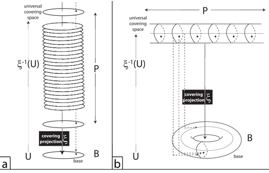
V.13.6 We can construct each of the distinct manifolds in the two covering spaces in Figure 34 into the base n times over simply by unfurling each one the desired number of times. And contrariwise, we can create the entire covering space simply by gluing together n copies of each of those bases.
V.13.7 Figure 34a’s covering space is a simple stack of pancakes. Every point in every pancake in the stack suitably covers a given point in the base. And if we undertake the reverse ξ-1 projection from the base upwards, we will find an appropriate point in every one of the pancakes purporting to be a covering for that base.
V.13.8 Figure 34b’s covering cylinder is also a covering space, but this time for a torus. The infinitely many circles along the cylinder’s axis cover the infinitely many about the prime meridian. And meanwhile, the single horizontal line along the cylinder’s length covers the toroidal equator. Every point on the torus successfully maps to its cover upon the cylinder.
V.13.9 We have now guaranteed reproduction. The biological significance is that a covering space preserves all copies of the original intact. We can get the cover for all possible generations from any number of current ones; and we can get any current generation from any other; either before or after. All covers to one side, i.e. underneath our species, are now its past generations; with all those the other side being its future ones.
V.14.1 We may now have a covering space and a projection that guarantees reproduction, but we have still not equated our exact and inexact differentials of ∫dn = ∫dP = ∫dM = 0 and ∇Q = ∇ • Q = ∇ × Q =0 respectively.
V.14.2 We now let some circulation follow a given path, y, about the rotachoron’s surface, at the constant altitude, or radial distance, r. But instead of following its designated path, let some Subpopulation D first leave, and then return to, that stipulated y path. It exhibits a +dx and then a -dx to and away from y. That out-and-back expedition is immediately the constant loop s ◦ s-1 about y.
V.14.3 Subpopulation D’s out and back expedition is now very similar to the ones made by our three constraints of ∫dn = ∫dP = ∫dM = 0. It, also, sums to zero as ∫dx = 0.
V.14.4 The meridians upon Boy’s surface—which is now a covering space—are relationships between our various manifolds. They are the stases of the first, second, and third kinds as rates. They arise from the following interactions:
• The one-dimensional gradients along each of the rotachoron diameters of τt, τn, τm, and τp. The inexact differential ∇Q = 0 comes from τt and τn for the cycle.
• The two-dimensional divergences between each coupling to give τtn, τtm, τtp, τnm, τnp, and τmp. The ∇ • Q = 0 comes τtn and τtm interacting over the cycle to produce the quantities in the divergence.
• The two-dimensional curls also in τtn, τtm, τtp, τnm, τnp, and τmp. This is again τtn and τtm interacting over the cycle, as ∇ × Q = 0, but now setting the rate at which the Möbius strip is traversed.
• The three-dimensional curls of τtnm, τtnp, τtmp, τnmp. This is both τnmp and τtnmp establishing, between them, both the quantities and the time points at which values and properties for n, m, and p are produced all about the circulation, and as ∇ × Q = 0.
V.14.5 Every expedition any subpopulation might undertake about our circulation, even in our covering space, will create the two matching constant loops s ◦ s-1 that are its Whitney umbrella.
V.14.6 Each one-manifold is a braid-1 that lies about its midpoint. Each affects the others, with their collective midpoints being their common identity, and the deformation retract.
V.14.7 Since, by Meme 122, our biological mapping cylinder is now also a covering space, then the relationships between our manifolds will preserve all fundamental groups in both preimage and image.
V.14.8 When our Subpopulation D takes its expeditionary path, it has a greater number of transformations than does any Subpopulation C that sticks to the stipulated path, y. Subpopulation C therefore has an additional, and constant dx = 0 constraint … where Subpopulation D is less restricted and emulates our three constraints by only having to satisfy ∫dx = 0.
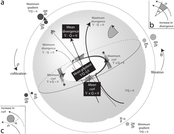
V.14.9 Since Subpopulation C is non-expeditionary, it has the shorter journey. And its movements are also across a projective plane. So when Subpopulation C holds constant, then as in Figure 35b it defines a Möbius strip midline.
V.14.10 Subpopulation D’s constant loop expeditions, out to each side of Subpopulation C, then define the Möbius strip journey all about that axis.
V.14.11 Since every Möbius strip bounds an area, then each must involve two dimensions. Subpopulations C and D must therefore be defining some twisting xy, yz, or xz plane for Boy’s surface.
V.14.12 And additionally … given that Subpopulation C maintains the Möbius strip axis value, it can also create Figure 9’s right helicoid.
But since Subpopulation D oscillates between a minimum and a maximum value, then it cannot form a right helicoid. It must instead move first closer to the helicoid axis, and then away, all about Subpopulation C’s white centre line.
V.14.13 As in Figure 35c, the Whitney umbrella’s constant loops, s, make a definite contribution to the overall circulation. Each has a definite and proportionate circulation density. That is its curl at that point.
And since all movements on each constant loop away from the identity increase the net contribution, they have a positive curl; with those inwards and towards the identity having a negative one because they decrease the net contribution. An in and out about a Whitney umbrella loop therefore sums to zero. All the V0 events are summed up by the constant S0.
V.14.14 If every span, x, about some circulation, τ, makes the same overall contribution to its circulation, then the curl is everywhere zero. But if any span x again makes a greater contribution either than the average, or else than its partnering complement or inverse of x’ and/or x-1, then that x has a positive curl; and if the converse, then it is negative. If it returns to its start point then its expeditions again sum to zero.
V.14.15 We now propose a Subpopulation A. It is a rotahedron. It pushes its three values right across the rotachoron’s diameter. It thereby constructs one of the four spherindrical diameters.
That Subpopulation A spherinder holds fast to the values that Subpopulations C and D will each restore when they have completed their circuits about the rotachoron’s surface, and have arrived back at the self-intersection point. It therefore passes straight through the deformation retract and Boy’s surface triple point of τ’t’.
V.14.16 Our Subpopulation C is now a cubinder upon the rotachoron’s surface, and all about Subpopulation A’s spherindrical diameter.
Subpopulation A also defines both (a) the helicoid axis, and (b) the central midline about which Subpopulations C and D oscillate.
V.14.17 As a further clarification of these various four-dimensional interactions, then Accra and London are both within a few degrees of the prime meridian. Since Subpopulation D’s expeditions about that journey will carry it off the prime meridian, it will go to various locations about the surface. Its path is again automatically longer than Subpopulation C, which always takes the direct journey straight down the prime meridian.
V.14.18 Subpopulations C and D both, however, take a longer path than Subpopulation A, which is at the centre of the earth’s crust, mantle, and core. Subpopulation A’s route is the path taken by the earth’s centre, as it is carried along its orbital path. Its equivalent Accra–London journey is the projection down from Subpopulations C and D onto that centre-holding path from τ-1t-1 to τ1t1.
V.14.19 There is, however, a specific relationship between Subpopulations C and D and their surface journeys. Subpopulation C’s non-expeditionary journey is the self-same journey Subpopulation D would be undertaking if only Subpopulation D was successful in negating every acceleration being imposed upon its windwalls and recurvatures. But since Subpopulation C does exactly the negating of accelerations that D refrains from, then C successfully follows its distinctive prime meridian and surface path.
Subpopulation C successfully instigates an s-1 counter loop for every s loop that the surface—or other atmospheric exigencies—seeks to impose. And since every surface location Subpopulation C and its windwalls and recurvatures pass through has a constant loop that confirms the prime meridian, then in successfully countering all possible deviations, Subpopulation C will always have a shorter path than Subpopulation D.
V.14.20 Where Subpopulation C successfully follows its constant meridional path, Subpopulation D instead exhibits Figure 35b’s Möbius strip increases, and then decreases, about C. However, the two subpopulations always have the same latitudinal Accra–London divergence. Subpopulation C defines the Möbius strip axis and right helicoid path about which Subpopulation D then deviates. And since Subpopulation C sticks rigidly to the prime meridian, then its longitudinal divergence is always zero … wheras Subpopulation D always adds and/or subtracts longitudinal divergences to itself.
V.14.21 Subpopulation D’s nonzero longitudinal divergence is the rate of change of the area bound between it and Subpopulation C as they each move latitudinally about the surface on their Accra–London journey. As in Figure 35b, a positive divergence is the increase in that area. A negative one is its decrease. In the equilibrium situation of the stasis of the second kind, we have ∇ • Q = 0.
V.14.22 Subpopulation D’s divergences in longitude now mean that its expeditions about that Accra–London journey create a constant loop that swings it out first to one side of Subpopulation C, and then to the other, also creating a series of curls. And since every population is similarly characterized, then they all have similarly matched pairs of two-dimensional constant loops that diverge about some mean, acting as a meridian, to construct the entire rotachoron surface as a set of divergences and curls.
V.14.23 Every dimension can also create a three-dimensional curl. We have followed Euler and expressed all values proportionately, across the unit distance 0 to 1.
If the total period for some curl and/or constant loop and/or divergence is T, then it immediately covers 1⁄T in each second, which is the rate T seconds−1. So if the blue whale in Figure 33 is r times further away from its own deformation retract than is the insect from its, then the blue whale covers an area, for its divergence, in each second, that is er times as great. But the blue whale must also curl about its circulation equivalently more slowly again in each second, than does the mosquito, so it can undertake that greater divergence. Where the average mosquito has a circulation of τ = 4 days, the blue whale not only has τ = 31 years, but gains 91 kilogrammes, 200 pounds, in weight each day over its first year of life (Busia 2014). The Möbius strip boundaries and areas may be significantly larger for the one than for the other, but both sets of curls and divergence nevertheless increase and decrease to be zero, overall, over τ and T, so that we have the stasis of the third kind where ∇ × Q = 0.
V.14.24 And since every dimension can interact with two others in a three-dimensional curl, then there can be a Subpopulation B that pursues a route that changes the altitude, r. Subpopulation B can therefore evidence a rate of change for r that takes it beneath the surface. This is a negative divergence in height.
The negative divergence in height Subpopulation B undergoes is the effect of a gradient, -∇r. So while Subpopulations C and D are the same in maintaining altitude—which is by having no constant loop in r—Subpopulation B differs, from both, by adding such a constant r loop in its gradient to give ∫dr = 0.
V.14.25 The Seikan Tunnel in Japan—which connects the Aomori Prefecture on Honshu with Hokkaido—is the world’s longest and deepest undersea tunnel … although the Channel Tunnel that connects Folkestone in the United Kingdom, with Coquelles, near Calais, in France, has the longest undersea span. Both these are direct connections that link their surface points by providing shorter journeys, due to their changes in height, than do the surface journeys between those same two locations. They are changes along gradients.
V.14.26 If Subpopulation B pursues a route similar to the above tunnels, then both its gradient and its divergence in height are negative for the first part of its journey. That negative divergence and move along the gradient eventually take it to its maximum depth … which also signals its maximum separation from the surface. The divergence in height is then temporarily zero, because there is no change in height. The gradient, however, still exists. It still points in the same negative direction to the earth’s centre.
V.14.27 The divergence and the change in height both now reverse to become positive, but against the same gradient. We now have a positive gradient, of the same value, as Subpopulation B moves in the opposite direction for height, proceeding towards journey’s end.
The original height is eventually restored, all against the same-sized gradients as before. The net divergence in height at journey’s end—which is also the sum of all the changes in height—is again zero.
V.14.28 In addition to the above, the changes in height Subpopulation B experiences both are—and exhibit—a curl. If the descent along the gradient, to go below the surface, accompanies an overall rightwards journey about the earth’s surface, and so about the earth’s centre, then it is a positive curl; otherwise it is negative. And if the accompanying ascent tends leftwards then it is negative; otherwise it is positive. This component of the curl adds to, or subtracts from, any created by changes in circulation density or overall circulation length, τ. The curl is therefore normal to whatever two dimensional plane of activities holds the circulation intensity at that point, with its magnitude being the maximum at that point.
V.14.29 And then finally, since these gradients, divergences, and curls are all rates, then although any path, x, between any two points can be shorter than some alternate path, y, between the same two points, y can still end up being quicker by having the greater rates of change. If we, for example, drive a faster vehicle, then the journey along a more circuitous highway can easily be quicker. The faster vehicle means we can maintain a greater velocity or rate of change. But “quicker” simply means “shorter” in the fourth dimension, which has a greater rate of change. Since this is a four-dimensional rotachoron, we “burrow” “under” the temporal surface. The slower journey remains “on the surface”, and “up above”. We have different divergences and curls in latitude, longitude, and height … including in the temporal dimension. So if some journey on an ostensibly longer path indeed ends up being quicker, then that fourth, and unseen, dimension either has a shorter path in its direction, or else has a greater gradient, ∇, for that fourth dimension, and irrespective of the path’s apparently longer distance in any visible dimensions.
V.14.30 All these same issues of gradients, divergences, and curls will now hold for the longitudinal journey between Singapore and Nairobi. Since those two are within degrees of the equator, then a Subpopulation D journey will produce a nonzero constant loop, plus Möbius strip, that now show divergences in latitude about the partnering Subpopulation C which has none. It instead balances in its north-south wind wall and recurvature accelerations as it holds to its constant equatorial path, maintaining its divergences in latitude of zero while they share a longitudinal divergence. And a Subpopulation B can tunnel beneath them; or fly above them; while a Subpopulation A can track their movements relative to the earth’s centre. The Accra–London and Singapore–Nairobi circumstances in A, B, C, and D mirror each other with just an exchange of latitude for longitude and vice versa. Exactly the same holds over all four dimensions and diameters.
V.14.31 We can therefore relate our inexact differentials of ∇Q = ∇ • Q = ∇ × Q = 0 to our exact ones of ∫dn = ∫dP = ∫dM = 0 at any time whatever simply by using some ∫dx = 0 to relate the two in some appropriate dimension. That is in our case a four-dimensional rotachoron, and a real projective plane. Larger expeditions simply mean a larger V4 volume. So no matter what the sizes of those expeditions, they sum to create some rotachoron, which simply has a different overall diameter and volume, thus preserving all topological invariants, with that ∫dx linking them together.
V.15.1 We can equalize our stases of the first, second and third kinds with our three constraints by considering them in four dimensions. The gradients, divergences and curls create constant loops that vary over time as the one-dimensional gradients and spherindrical diameters of τt, τn, τm, and τp that we see in Figure 35’s rotachoron diameters. Their unseen τtn, τtm, and τtp divergences form the pole to pole gradients that are the values over time that establish the four spherinders, cubinders, and glomes. They together create the τtnmp circulations of the generations for each and every population. They help establish the three meridians of τtnm, τtnp, and τtmp that define Boy’s surface. These flatten with the τt hyperplane, at each absolute clock moment, t, to create the twisting nm, np, and mp surfaces that are the backbone for the Möbius strips. Those then participate in the bases, fibres, fibre bundles, and covering spaces that are all biology and ecology.
V.15.2 Möbius was the first to realize the implications of the real numbers, ℜn, we use to represent a point in n-dimensional space. In his 1827 work Der barycentrische Calcül (O’Connor & Robertson, 2015) he introduced the idea of “homogeneous coordinates” that would permit geometric calculations in all projective spaces.
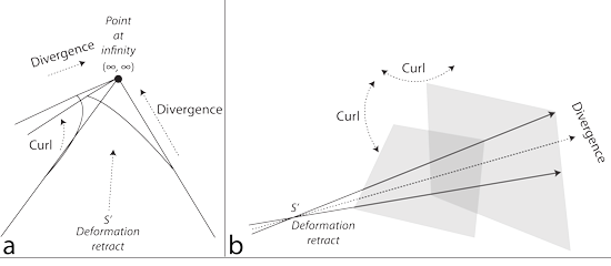
V.15.3 While two parallel lines upon an ordinary Euclidean plane go out to infinity, seemingly at a constant distance from each other, and so do not intersect, those on a real projective plane will have the perspective projection of Figure 36a that carries them to their meeting at the point at infinity. No matter where they might begin, or how much they might curl towards or away from each other, the divergences and curls do not change that tending to the same point at infinity, which is represented, in Euclidean coordinates, as (∞, ∞).
V.15.4 Each real projective plane is a hemisphere placed upon a plane. Its horizon line is at (∞, ∞). That is a unique point upon the real projective plane towards which all lines converge. Each is therefore a two-manifold whose global topology forms a curving V2 planespace, while its local topology forms the S2 planespace that tends it to infinity.
V.15.5 Möbius introduced an extra coordinate. Since each real projective plane is two-dimensional, we create homogeneous coordinates by representing each point on each line with the triple (x, y, w). So if we have three different lines, we can express any given point upon each as (1, 2, 4), (2, 4, 8) and (12, 24, 48). When re-expressed in ordinary Euclidean coordinates, each become (1⁄4, 2⁄4), (2⁄8, 4⁄8) and (12⁄48, 24⁄48). But these are all the same (1⁄4, 1⁄2) points in Euclidean space. They are thus the same relative point, no matter what their lengths or orientations.
V.15.6 We now have an equation of the form Ax + By + Cw = 0 for each line upon a real projective plane, with at least one of A, B and C being non-zero. The Cw, which is independent of both x and y, now allows any line to be transformed to any other. We simply determine Ax⁄Cw and By⁄Cw for any point transferred from one line or projective plane to another, and we recover the given point. There is the added advantage that a movement towards infinity is tending towards zero as a limit on all lines, which can now do so at their given rates.
V.15.7 Any (x, y, w) is now the same as any (αx, αy, αw). All points at any point on any one line, expressed in homogeneous coordinates, are equivalent to all points on any other. As long as A, B, and C are real numbers, with not all three being zero, then they describe the identical line on any projective plane.
V.15.8 We can now use the non-zero α to scale by any amount for any other projective plane. We simply multiply and divide by the w-coordinate. But since a real projective plane contains that extra zero coordinate, all the Euclidean points that tend to infinity cluster around the real projective plane’s zero point. If a population of ants ranges from say 2 to 6, while one of blue whales ranges from say 1 to 1,000,000, then even though they have different absolute sizes and values in their point-, line-, plane-, realm- and tetrapaces, the 50% point for the ants is 4⁄6 while that for the whales is 500,000⁄1,000,000, each on their respective projective planes.
V.15.9 We can similarly introduce a w-axis into our three-dimensional space to give the four numbers (x, y, z, w). As in Figure 36b, they will handle all divergences, and all curls for all possible Subpopulations A, B, C, and D. Origins exist upon all, but do not necessarily map to the same absolute locations in each. Lines map to lines, but parallel lines do not necessarily remain parallel. Homogeneous ratios still exist, but points may not map to the same specific points that preserve the same ratios in each. It is the homogeneous ratios that preserve all identities, scalings, and rotations across all four dimensions. They form a group. They do not necessarily progress at the same rates across all four dimensions, but they still sum as both ∫dn = ∫dP = ∫dM = 0 and ∇Q = ∇ • Q = ∇ × Q = 0 all about their respective circulations.
V.15.10 Every biological set X and Y forms an open set that abides by the “fundamental theorem on limits”. Each has the Bolzano-Weierstrass property, with every infinite subset having its contained limit point. Each is “sequentially compact” with every possible sequence in each having a convergent subsequence so that:
“If a function u has a limit l and c is a number, then cu has the limit cl.
“If u and v have the limits l and m, respectively, then u + v has the limit l + m.
“If u and v have the limits l and m, respectively, then uv has the limit lm.
“If u and v have the limits l and m respectively, and if m is not zero, then u⁄v has the limit l⁄m.
“If u never decreases and there is a number A such that u is never greater than A, then u has a limit which is not greater than A.
“If u never increases and there is a number B such that u is never less than B, then u has a limit which is not less than B (James and James, 1992)”.
V.15.11 Every population can now scale, using itself as a unit. They all now transition between their points at infinity on each side, all tending to zero as a limit. Their multiplicative inverses and antipodal points will have both squares and absolute values that can tend infinitesimally closely towards zero for each, as the point at infinity, and no matter how much they are each scaled. They all now have additive and multiplicative inverses for all vectors, along with dot and cross products. A move to infinity is simply a move towards zero. The move in each towards a midpoint and/or equator is the move towards a snipped crossing point.
V.15.12 Every circulation is now equivalent to every other. Each becomes a circle that passes neatly through the point at infinity. They all have their equators and meridians. Each circulation is therefore divided into four quadrants, with each having a specific relationship both to each hemisphere and to the horizon, again differing only by scale. And for every unique line passing through two distinct points on any projective plane, then there is also a unique point lying at the intersection of two distinct lines. The same holds on all planes. The projective plane therefore makes all 0 to 1 expressions equivalent, with an expression or transition in any one being identical to that in any other, again irrespective of scale; and all about the circulation.
V.15.13 Since all coordinates represent the same basic point, then if a population of ants does not access some given point on its specified real projective plane because it is biologically impossible for it to do so, then since the points are expressed as a set of divergences and curls, the population will still not access those points when scaled to become comparable to a whale; and conversely. Every population’s transformations on every projective plane are therefore unique. They are independent of scaling. They all preserve all identities, all gradients, all divergences, and all curls.
V.16.1 There are now some consequences to Meme 122’s fusion of a biological mapping cylinder with a covering space. Our exact and inexact differentials must manipulate the same Euler characteristics, χ, and deformation retracts, S’, for the preimage and progenitor domain, X, and image and progeny codomain, Y, and so that they are bijective, with every point x in X able to substitute itself for y in Y and conversely. Each must be first base then fibre so that their joint product space P = B × F is their mapping cylinder, Mλ. They must both be simply connected.
V.16.2 Each meridian on Boy’s surface must have projections that are locally homeomorphic. All loops—both trivial and nontrivial—can be lifted to each of their covering spaces, preserving all possible transformations.
V.16.3 Each of X and Y when acting as either base or fibre, and therefore each projection, forms a simply-connected surface for the Mλ mapping cylinder. And since the covering space from which they each derive, and that they then form, must also be simply-connected, then every population has its unique “universal covering space”, C.
V.16.4 The unique universal covering space, C, is also the mapping cylinder, Mλ … and therefore the surroundings:
• We get the base’s π(S) = 0 fundamental group, and all its trivial loops, from a genus g = 0 universal covering sphere in C.
• We get its π(S) = Z2 fundamental group, and all its nontrivial loops, from a g = 1 universal covering plane which folds into a cylinder for a torus and for our equators again in the universal cover, C.
• We get its π(S) = Z2 fundamental group, and all its identified points for all minimum to maximum traversals, by procuring another universal covering sphere. We cut it in two at its equator; duplicate its northern hemisphere; rotate that by 180º; and reattach. We then have the doubly winding cyclic groups of order two, once again in the universal cover, C.
We can thus procure all the fundamental groups we need for the progenitor domain, X, and progeny codomain, Y, that jointly make the base, B, from the universal covering space, C, that is also both (a) the mapping cylinder, Mλ, and (b) the surroundings.
V.17.1 Each manifold can form a gradient such as ∇Q = 0 which defines some mean throughout its base space, B. It is also the foundation for the fibre in all bundle and cover contributions.
V.17.2 Since each manifold’s one-dimensional deviations about its own mean must be observed in the surroundings, then they are the τtn, τtm, and τtp recursive function values to which we can apply t as a cutting hyperplane to produce our loops that define the circulation for a generation. This then gives all initial and final values for n, m, and p over a generation. Each set of values can diverge as its braid-1. Each can be projected both into and out of the universal covering space, C; and so in and out of each set of progenitors, X, and progeny, Y, that is our base, B.
V.17.3 But each one-manifold also conjoins with others to form the two-dimensional divergences and curls that range between some minimum and some maximum as the three sets of paired and twisting Möbius strip values flattened, by t, from τtnm, τtnp, and τtmp to be observed as nm, np and mp. Their oscillations establish biological attributes over time and space for all bases, bundles, and universal coverings in each biological space S. They define the sizes and dispositions of Boy’s surface for a generation, again in the universal covering space, C.
All four manifolds also come together to create the τtnmp rotachoron. And once that has been flattened by a t hyperplane, it states the deformation retract and mapping cylinder values for the n, m, and p maintained at each point t over the generation. Their three-dimensional curls intersect to define each others’ rapidities and directions at each successive point about each base, and each fibre … and so once more throughout the universal covering space, C.
As again in Figures 34 and 35, the projections of these gradients, divergences, and curls create the surfaces that are the bases for any current population and generation. They then project back into the universal covering space, C, to help define that species.
V.17.4 By Meme 123, our mapping cylinder, Mλ, is also a universal covering space, C.
V.17.5 Since our mapping cylinder and universal covering space are now identified, then the three constraints require that the progenitor domain and the progeny codomain each act, by turns, as preimage and image, and so as bases, fibres, fibre bundles, and covering spaces.
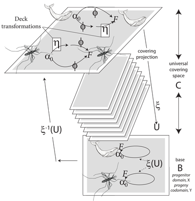
V.17.6 We also now require, as in Figure 37, there be a one–to–one correspondence between the covering projection of ξ that sends down from the universal cover, C, into some open set, U, in the base, and the reverse mapping, ξ-1, that sends back from the base into the universal cover, therefore acting as a fibre.
V.17.7 The progeny now loop, in the base, from their initial state, α0(B), to their terminal one, F(B). That F(B) is then identical to the α0(B) start point for their own progeny. And since the base interacts directly with the surroundings, then each base necessarily has transformations independent of those in the universal cover, C, projecting down into it. These are the stases of the first, second, and third kinds.
V.17.8 The universal covering space, C, covers all possible bases, B. It therefore has a far greater number of transformational possibilities than can exist for any single base. Those universal cover transformations must therefore be independent of all those occuring in any one generation, or any one base. Each distinct base must therefore be injective, ![]() , into the universal covering space; while the universal covering space is surjective,
, into the universal covering space; while the universal covering space is surjective, ![]() , over each distinct base.
, over each distinct base.
V.17.9 Since the universal cover’s surjective projections must remain unaffected by all returning injective fibres, then as in Figure 37, all universal cover transformations, such as φ, must remain unaffected by whichever inverse ξ-1 transformations are currently being sent back, along some fibre, and by some particular progenitor domain or progeny codomain. So any φ moving in the universal cover, C, from some initial point, α0(C), to some final point, F(C), must remain able to project the same transformation down into the base. It must identically benefit all possible bases and populations in their α0(B) to F(B) loops, and no matter what inverse ξ-1 arrives back, into the universal cover, from the base.
V.17.10 Let there now be some second—and so equally surjective—transformation, η, in the universal covering space. When we apply both it and φ to α0(C), we still end up—unchanged—at F(C), and no matter what the injective ξ-1(U) fibre arriving. It has the identity property. It acts so that η ◦ φ = φ ◦ η = f.
V.17.11 In 1897 Siefert and Threlfall (1980) first referred to such identity transformations as the Deckbewegungsgruppe or the ‘covering–movement–group’. They are therefore known as “deck transformations”.
V.17.12 As again in Figure 37, deck transformations are those identity transformations, within the universal cover, that can both (a) remain unchanged in that cover; and (b) project themselves—as if like a stack of playing cards—through endlessly many covers to arrive—unchanged—in the base.
For every ξ projection down into the base from the universal cover, a deck transformation exists that allows the cover to undertake a homeomorphic transformation that matches whatever transformations the base might care to undertake, after first receiving that projection, and then projecting its own resulting state back up into the cover, along its ξ-1 fibre, as a reverse projection to arrive back in the universal covering space.
A deck transformation effectively lifts back up into the universal cover whatever projection was previously sent down from the cover, and no matter how it might have been transformed within the base. Every path and loop in every base can therefore lift up into the universal cover to create the precisely matching beginning and endpoints α0 and F for that returning path and loop, for it has been left unchanged upon both arrival and departure. No matter what transformations any base might undertake as it interacts with the surroundings, the deck transformations maintain a universal cover integrity.
V.17.13 Deck transformations state the symmetries within the covering space. They preserve all projections and inverses by mapping the universal cover’s identity operations. They therefore ensure a one-to-one mapping between the base’s fundamental group and the ξ-1 fibre or inverse projection that lifts from each distinct base into the universal cover.
V.17.14 Deck transformations also ensure that the universal covering’s deck transformation group, η, are isomorphic with the base’s fundamental group, π(B). They form a Galois group.
V.17.15 Since the deck transformations permute every fibre lifting from every base to create their η ◦ φ = φ ◦ η = φ, then they guarantee the homeomorphism of both the progenitor domain, X, and the progeny codomain, Y, as preimage and image; and conversely. They can project through infiinitely many covers into the base and still guarantee that base’s behaviours … whilst simultaneously allowing all bases to reciprocally lift all possible subsequent transformations back up into the universal cover, and no matter how frequently they might be repeated. They hold invariant in the face of all permutations in inexact differentials, of whatever type, transmitted up into them. The universal covering space’s exact differentials therefore remain supremely indifferent to them all.
V.18.1 Since the universal covering space, C, is also the mapping cylinder, Mλ, then the rules for biology and ecology reduce to the rules that govern (a) those deck transformations; and (b) the fundamental groups in the base. Those are (a) the identity, η, in the cover operations; and (b) the complete set of transformations involving π(B), which must now be all possible Chomsky production rules within the mapping cylinder, Mλ.
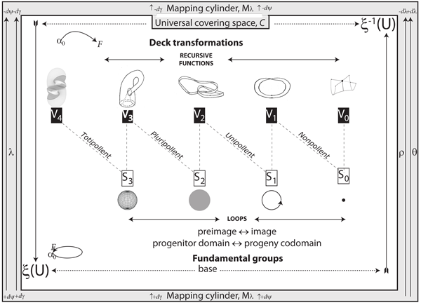
V.18.2 As in Figure 38, the universal cover pulling up as the ξ-1 fibre from the base is also the mapping cylinder lifting as the fibration, θ. This is the combination of +γ and +ψ moving between base and surroundings as the +λ biology and ecology entering the plessists and plessemorph through their +r inputs.
V.18.3 The universal cover projecting down as ξ is the mapping cylinder lifting as the cofibration, ρ. This is the combination of -γ and -ψ moving between base and surroundings as the -λ biology and ecology departing the plessists and plessemorph through the -r outputs.
V.18.4 By Meme 124, since our biological spaces conform to both the three stases and constraints then they are interacting with the surroundings to form metric spaces.
V.18.5 Since our biological spaces are metric, then they are immediately “Hausdorff”. Named after the German mathematician Felix Hausdorff, a “Hausdorff space” always contains both the entire set and the empty set, ∅, amongst its infinitely many open sets, U.
An “open set” in a Hausdorff topology means we can, for example, take any two sets that form two S2–V3 rotahedrons, and so that satisfy the general equation, x2 + y2 + z2 = r2. Each then has infinitely many points, within its boundary, that satisfies its equation, and that fall either upon, or within, its defining bounds. Each such set can form infinitely many V3 or 3-ball, subsets. Each of those subsets can also include the entirety of its V3. Each set’s empty set, ∅, also falls within its respective S2 boundary.
A Hausdorff space means that the union, ∪, and intersection, ∩, of any finite number of open sets is also always open in the sense that there are infinitely more such sets within each set of bounds that can satisfy that space’s description. And since they all abide by the fundamental theorem on limits, we can always get infinitesimally closer to any and all of them.
A Hausdorff space defines the discrete collections of homomorphic points that are our distinct biological entities. Any two distinct points or collections of points in any Hausdorff space—such as with our plessists, plessemorphs, and other biological entities and that inhabit our biologically metric spaces—can be separated from any other.
V.18.6 Since our t-, n-, m-, and p-manifolds are all metric, and therefore Hausdorff, then every point in each is contained in an open set that is always homeomorphic to the real numbers.
V.18.7 Each set U is always open in each of X and Y. All functions and images φ:X → Y and φ:Y → X go to a U(X) and a U(Y) in each. Their inverses φ−1(U(X)) and φ−1(U(Y)) are also open and continuous.
V.18.8 If p and q are plessists and/or plessemorphs—which means distinct points or groups of points—we straight away have the disjoint open sets U(X(p)) and V(X(q)) in X, and U(Y(p)) and V(Y(q)) in Y. They are each separate sets.
V.18.9 As now required, there exist neighbourhoods in both X and Y around p that do not contain q; while there exist neighbourhoods around q that do not contain p. All progenitor and progeny sets and subsets are therefore open. Any union is open. Any finite intersection of open sets is again open.
V.18.10 Every countable open cover of each has a finite subcover. Both X and Y are countably compact and equipollent with the natural mumbers.
V.19.1 By Meme 101, our biological structures are locally indistinguishable homomorphic groups of points that reside on and are composed of manifolds, whilst our homeomorphisms, being collections of such groups, can define the global spaces those points occupy.
V.19.2 Every interaction between a progenitor domain, X, and a progeny codomain, Y, is a biological homomorphism between groups of points as entities. It is some mapping φ:X →Y. It must also be continuous. Since it must be moving from the universal covering space, C, into the base, B, it may not be one-to-one. It is therefore a surjective mapping, or onto.
V.19.3 There must also be a reverse mapping from progeny codomain back to progenitor domain as φ−1:Y → X. It must again be continuous. And since it cannot be onto, it is an injective mapping, or one-to-one.
V.19.4 Since one of these mappings is injective, the other surjective, then X and Y must be homotopically equivalent.
V.19.5 Since we have both a homomorphism and a homotopic equivalence between the progenitors, X, and their progeny, Y, then they both map between 0 and 1. We have the two continuous functions φ:[0,1] → X and φ:[0,1] → Y, respectively, and so that for every pair of points a and b in X, and c and d in Y, then a = c = φ(0); and b = d = φ(1).
V.19.6 We also have direct and one-to-one mappings to and from each of X and Y, and to and from both the mapping cylinder and the universal cover. Their deck transformations and fundamental groups must therefore be isomorphic.
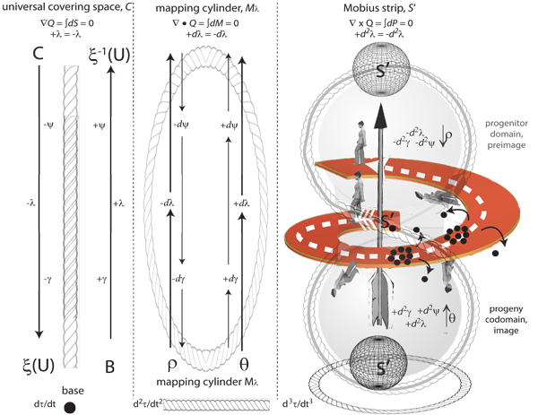
V.19.7 Figure 39 shows the different one-to-one correspondences we can build between the base, B, on the one hand, and the universal cover and mapping cylinder, C and Mλ, on the other. For every point we see in the base, which is any value in time, there is a dynamical exchange between +r and -r through the Whitney umbrella in the cover. The same point is at one time an input as the surjective C → ξ(U); and then it is an output, with the same value, as the injective B → ξ-1(U). This change occurs at a given velocity, and also equates the first and second stases which are the gradient and divergence in numeracy, ∇Q = ∇ • Q = 0. Then for every line we see in the base, which is any unidirectional change maintained over time as either C → ξ(U) or B → ξ-1(U) and so which is a trivial cycle, there is a circulating journey from minimum to maximum and returning that is a nontrivial cycle, and that also aligns some deck transformations with the base fundamental groups. This further equates the first and third stases of the gradient and the curl in numeracy, ∇Q = ∇ × Q = 0. And then for every nontrivial journey in the base and so across a real projective plane, there is an accompanying journey about a Möbius strip as the conjoined ξ projection down from cover to base and the ξ-1 back along fibre from base to cover that equates all three stases of gradient, divergence, and curl in numeracy: ∇Q = ∇ • Q = ∇ × Q = 0. This is a circuit about both sides of Boy’s surface. It is equivalent to, for example, a given person being taken blindfolded around a given circuit on a first occasion … which is repeating on a second occasion, but with the blindfold removed. So while the circuit is repeated twice over, the individual concerned believes it to be but a single circuit conducted in two different states.
V.19.8 Since we can use the real numbers, ℜ, to describe all our paths in X and Y, then they are by definition connected. And if X and/or Y are indeed connected; and if φ is a continuous function from X onto Y and Y onto X; then each one is mapping to the other while also being connected. We now have discrete collections of homoemorphic points that are the paths in any Hausdorff space.
V.19.9 If p and q are distinct paths in each of X and Y, we straight away have the disjoint open sets U(X(p)) and V(X(q)) in X, and U(Y(p)) and V(Y(q)) in Y. They are each separate sets. There is a neighbourhood in each that does not contain any paths and points in the other. Any union and finite intersection is also open.
V.19.10 And … we at long last have a statement not just about the functions or mappings, φ, and so not just about the homomorphisms within X and Y. We have here a statement about the spaces. Both the spaces X and Y are “path-connected”. They are therefore potentially homeomorphic spaces that contain homeomorphic groups of points.
V.20.1 Although it remains impossible to show four dimensions in only three, Figure 39 depicts the consequences of the interactions between the base, B, the mapping cylinder, Mλ, and the universal covering space, C … with the progenitors, X, and progeny, Y, being the base; and the surroundings being the mapping cylinder and universal covering space conjointly.
The universal covering space, C, in Figure 39a uses its deck transformations to project ξ into the base at the rate dτ⁄dt. It guarantees the XX’, XX-1, YY’, and YY-1 constant loops, complements, and inverse couplings of s ◦ s’ = s’ ◦ s = τ and s ◦ s-1 = s-1 ◦ s = S’. Those plessists that can remain sufficiently close to each other, and to these S’ values, will produce the next generation that can then repeat the process.
V.20.2 Figure 39b has the lifting of progenitor domain as preimage, into the mapping cylinder as a fibration, θ, and as a set of biological interactions. We begin moving from α0 to F. We have a set of γ and ψ biological-ecological interactions. They are also a part of the deck transformations, η.
As these same deck transformations then continue to their terminal point F, so do all the transformations in the mapping cylinder gradually reverse. They become the cofibration ρ, and a further set of γ and ψ interactions in the surroundings, again lifting to the mapping cylinder. These are also the ξ-1 reversals projecting from base back to the universal covering space. The total is both the deck transformation identity, η, and the biological–ecological transactions, λ. They occur at the rate d2τ⁄dt2.
V.20.3 We see the same transformations in Figure 39c which depicts a helicoid, a spherinder, and a Möbius strip as the population moves about our biology and replication globes. It moves from an initial location, α0, in the universal cover out towards F. The entities are guided all about the Möbius strip by their Whitney umbrellas. They occur at the rate d3τ⁄dt3.
V.20.4 There is also a set of transformations—overseen by the fundamental groups in the base—looping from α0 towards F, but as the set of changes S-1, about the helicoid, heading towards S0 in the mapping cylinder. A spherindrical journey from pole to equator is equivalent to a Möbius strip loop towards the crossing point that is the deformation retract, S’.
V.20.5 While the total of the biological-ecological processes is λ, the circulation length is τ. The absolute clock time needed to traverse them is T. The θ, ρ, γ, ψ and λ operations again proceed along the length in Figure 39a at the rate dτ⁄dt; they have dλ increments about Figure 39b’s unknot at the rate d2τ⁄dt2; and d2λ increments around Figure 39c’s Möbius strip at the rate d3τ⁄dt3.
V.21.1 If we express the points in each of X and Y more generally, as p, q, and r, then we can create a set of homogeneous coordinates that will allow us to scale any population to any other by expressing the four values (p, q, r, w) as (αp, αq, αr, αw), as long as α is non-zero.
We can alternatively use Ap + Bq + Cr + Dw = 0. As long as at least one of the coefficients is again non-zero, then we can use Dw as the independent value that transforms as Ap⁄Dw, Bq⁄Dw and/or Cr⁄Dw.
Granted that in ‘8⁄4 = 2’ we call 8 the “dividend”, 4 the “divisor”, and 2 the “quotient”, then the Dw in the above is acting as a “divisor” on the whole biological space. Our dividend is in this case an entire circulation of the generations. That Dw is a constant that helps determine the space’s size and characteristics.
V.21.2 The entities at any point in our X and Y spaces form the subspaces U(X) and U(Y). But if the generation is to continue, then there must exist other spaces that are intrinsically biological, and so at least potentially within the overall X and Y, that entities can enter, but that are still outside their current and designated U(X) and U(Y) subspaces.
V.21.3 We can identify those potential spaces the population can enter by taking U(X) and U(Y) as divisors. Our dividend is then the entire circulation of the generations. The space we define is outside any current U(X) and U(Y), but still preserves both ∇Q = ∇ • Q = ∇ × Q = 0 and ∫dn = ∫dM = ∫dP = 0.
V.21.4 Any subspace in each of U(X) and U(Y) can take itself as a divisor for the whole. It then creates a “quotient space”. And since that quotient space must always exist; and further since it is characterized everywhere by having the same Dw as its divisor; then the space holds that given divisibility property in common. It is their common divisor. It is therefore also called an “identification space”.
V.21.5 Our identification space is outside any current points and collections of points as either paths or functions … but is still uniquely accessible to all such points by being a part of their shared identification space. It is again the common dividend for all their divisors to produce their given quotients.
V.21.6 Since the identification space is characterized by sharing the same divisor everywhere, then it must have some form of “equivalence relationship”, ∼.
V.21.7 This ∼ equivalence relationship characterizes the space as capable of supporting whatever transformations either will be undertaken, or have been undertaken, by the points currently in U(X) and U(Y), and so that they can either become, or else revert to being, points in that identification space.
V.21.8 Our topological spaces X and Y must bear this ~ equivalence such that if some set U is open in that identifcation space, then its inverse mapping, say s−1(U), back into X and Y is indeed open. Both U and s-1(U) must therefore always be open sets in both X and Y.
V.21.9 If we deformation retract any current U(X) and U(Y) subspaces down to a single point, then the remainder is the quotient or identification space. It must share that equivalence relationship, ∼. And since the equivalences are quotients, then they are ‘X⁄∼’ and ‘Y⁄∼’ respectively.
V.21.10 Our Whitney umbrella and π(S) = Z2 fundamental group stipulate that for every p in X⁄∼ and Y⁄∼ there exists a q that is the same as p, excepting only that it has a change in sign. Our equivalence relationship is therefore p = ±q.
V.21.11 We can now say that for any point p in any U(X) or U(Y) we always have the “structural equivalence”, p ≈ q where p = ±q. The whole of our space therefore has the structural equivalences:
• p ≈ p, which is a reflexive structural equivalence;
• if p ≈ q, then q ≈ p which is a symmetric structural equivalence;
• and if we have both p ≈ q and q ≈ r, then we have p ≈ r which is a transitive structural equivalence.
V.21.12 This p ∼ q equivalence identifies all points throughout the identification space, but as behind their common boundary. It creates the set of open equivalences U and s-1(U) all across both X⁄∼ and Y⁄∼. And since our structural equivalence is always some p ≈ q, then we can partition X and Y into p and not-p, where not-p ≡ (-p, ±q). The entire not-p space is identified by that structural equivalence.
V.21.13 We now have an open identification space that defines the boundary common to both (a) all ps, and (b) all the not-ps that can nevertheless transform into ps. And since for every p there must exist some -p, then those two can always produce the identity.
V.21.14 Identity creation is the structural equivalence throughout our identification space. It holds throughout X⁄∼ and Y⁄∼. All points throughout any X and Y share that same identity.
V.21.15 We can in particular note that the sets of points in X and Y that do not have this structural equivalence of +p and -p coming together to produce a common identity is zero. Our identification space is uniquely identified by its identity, S’.
V.21.16 Our identification space successfully identifies all points opposite to all others. Each identification space thereby gives us all the neighbourhoods accessible to any point in either X or Y when either preimage or image.
V.21.17 And since the X⁄∼ and Y⁄∼ spaces guarantee that we can find all opposite values for all constant loops, inverses, and complements, then we have a compact and connected projective space that contains both an identity as a crossing point, and a Möbius strip.
V.22.1 Since our spaces are Hausdorff, path-connected, and now identified, then we can define each X that deforms to a Y with that Y deforming back to X and conversely as a “zone of reproductive accessbility”. This is also our conjoined identification space, X⁄∼ and Y⁄∼.
V.22.2 Each XY coupling establishes a set of biological homeomorphisms by establishing both the paths and the boundaries that define biologically replicative populations and spaces. We simply let {Xα} be a set of connected—and therefore path-connected—subspaces in X whose union is all of X; and we let {Yβ} be a set of connected—and therefore path-connected—subspaces in Y whose union is similarly all of Y. Each space can therefore be both (a) a complete population, and (b) a generation. And if Xα1 ∩ Xα2 and Yβ1 ∩ Yβ2 are each nonempty over all possible indices, then the two spaces are each both (a) connected; and (b) path-connected.
V.22.3 If our X and Y spaces are each indeed connected, path-connected, and identified as X⁄~ and Y⁄~, then we can bring them together to create a joint X × Y or product topology. This immediately has a base B under the following conditions:
• B ≡ BXY ∪ BYX;
• BXY ∩ BYX is not empty;
• BXY = {U(X) × V(Y) | such that U is open in X and V is open in Y};
• BYX = {U(Y) × V(X) | such that U is open in Y and V is open in X}.
V.22.4 We now have the subsets U(X), V(X), U(Y), and V(Y) throughout X × Y and Y × X that are all properly Hausdorff, open, and nonempty. We also have their respective unions U(X) ∪ V(X) = X and U(Y) ∪ V(Y) = Y.
V.22.5 However … the full generality of all the sets that could be formed in either of the product topological spaces X × Y or Y × X is not necessarily always open. Indeed, we do not necessarily always form either, or both, of those products.
V.22.6 But since our spaces are explicitly Hausdorff, for all biological entities have definite sizes and measures, then we certainly have the intersections of U and V in each of X and Y. And if those intersections produce the empty set so that U(X) ∩ V(X) = ∅ and/or U(Y) ∩ V(Y) = ∅, then whichever one of X or Y has that empty set intersection does not have a path-connection, and so is suitably “disconnected”. We do not have B = BXY ∪ BYX, and/or BXY ∩ BYX is empty. The X × Y product space may be homotopic, but it is now not homeomorphic. We do not then have the full two-way transformations that define a fully viable species. We either have non-compatible parents that produce a non-viable hybrid, or fully compatible parents that produce non-fertile progeny.
V.22.7 We can now say that if ever either—or both—of X or Y acting as either preimage or image is disconnected, in the above sense, then either only one of BXY and BYX exists, or else neither does. Since we do not have both, then one or the other, or both, of X or Y is disconnected. The disconnected one is either not biological, not replicative, or it is neither. Either one, or both, of θ and ρ fail to lift to the mapping cylinder; and either ξ is not received from the universal cover by the base, or else ξ-1 is not transmitted by the base to the cover, or else both. That disconnection means one or the other of BXY or BYX is empty so that we do not have the full base, B.
V.22.8 But if either X or Y is not disconnected, then each is by definition connected. And if both X and Y are connected—so that we have both BXY and BYX, and both ξ and ξ-1, and both θ and ρ—then we have a non-empty basis, B, which acts on both sets of mappings X to Y and Y back to X. This doubling of space connectedness and path-connectedness gives us the biological double of (a) homomorphism and (b) homeomorphism. It defines both of the non-empty XY and YX product spaces over an entire generation. We then have a viable population that can also form a clear species.
V.23.1 Since our biological spaces X and Y are both now Hausdorff and metric, then they together give us a determinable and measurable zone of reproductive accessibility. That zone is defined by the properties projected, as progenitors and their progeny, between the universal covering space, C, and the mapping cylinder, Mλ. It produces a finitely countable set of plessists, plessemorphs, and/or biological entities as can together create π.
V.23.2 All the original points x in any progenitor domain X of this kind can now take the surroundings as both their mapping cylinder, Mλ, and universal covering space, C. They can use an index i to map themselves into a progeny codomain as the points y in Y, but with Y being the deformation retract. This is then the universal cover that projects surjectively as ξ down into the base. It is also the cofibration, ρ, lifting from X into the mapping cylinder, and as part of the overall biological-ecological processes, λ.
V.23.3 All of the points y in Y that result from the x in X can now use the same mapping cylinder, Mλ, and universal covering space, C, to map in reverse as ξ-1, lifting back from the base into the universal cover; with X now in its turn being the deformation retract to Y. This is also the fibration, θ, lifting up to the mapping cylinder in the same biological-ecological processes, λ.
V.23.4 One of those two sets X and Y is now the direct progenitor to the other. It lifts plemes and plessetopes, and plessiomes and plesseomes, as ψ and γ, respectively, into the mapping cylinder as ρ, while receiving them, surjectively, as ξ into the base. The other is the direct progeny, again lifting plemes and plessetopes and plessiomes and plesseomes, as ψ and γ, into the mapping cylinder as θ; but simultaneously injecting them into the universal covering as ξ-1.
V.23.5 If, however, there is no basis, B, with suitable path-connectedness in both directions as BXY and BYX, then although both sets X and Y may be biological, ecological, and homomorphic as λ =(θ, ρ, dθ, dρ), there is no shared zone of reproductive accessibility. They do not share a set of increases plus decreases in ψ and γ in their common product space, and so there is no homeomorphism and no viable species. We now have some clear definitions.
V.24.1 We have now defined all of biology and ecology. It is the biological journey across a rotachoron from pole to equator to opposite pole over some period of absolute clock time, T; as well as the journey from the deformation retract S’ = (n’, m̅’, p̅’) that is the contact point between the biology and replication globes about both of them to return from the same direction and so about a Möbius strip of length τ.
V.24.2 The above journeys also creates the four spherindrical diameters τt, τn, τm, and τp plus three meridians τtnm, τtnp, and τtmp that create Boy’s surface. This again has τnmp centred upon τ’t’ for its triple point, which creates the rotachoron by sustaining S’ over both τt and T.
V.24.3 The replicators that our Hausdorff and topological spaces have provided are open sets. They create an identification space behind the definite s ◦ s’ = s’ ◦ s = τ and s ◦ s-1 = s-1 ◦ s = S’ boundaries. The former is the total distance about the generation, the latter states the distances between the states maintained by defining their centre.
V.24.4 Since the Möbius strip journey begins and ends at the crossing point, then τ is a vector. It measures the displacement from that crossing point, which is the total journey about both globes.We must, however, change in direction twice, which is a set of both (a) jerks or triple derivatives, and (b) accelerations or double derivatives.
V.24.5 And … we have now corrected Dawkins’ problematic usage of “open-ended” when insisting on “tight discipline” in describing “true replicators” for a “Darwinian model” (Dawkins 2004). Those shared increases and decreases in γ and ψ that create the biological-ecological activities λ define the mapping cylinder, deck transformations, and universal covering space. Progenitors and progeny can vary topologically with their open sets, but always whilst creating a surface that abides by specific rules, and through a potentially infinite number of generations.
V.24.6 We can now state those specific rules. They are (A) the three constraints; (B) the four maxims of ecology; and (C) the four laws of biology.