VI.1.1 We can now use our S3–V4 rotachoron, the four-dimensional interactions from Boy’s surface, and the identification of the mapping cylinder with the universal covering space to deliver the three constraints, four maxims, and four laws that explain all biology and ecology:

The purpose of a model is to summarize knowledge, support insights, make hypotheses explicit and quantitative, and predict or explain new phenomena. Although each aspect of a movement can be explained by many models, the requirement that a single model account for as much normal and abnormal behaviour as possible constrains the choice of models and reveals isomorphisms that contribute to our understanding …. (Ramat, Leigh, Zee, Optican 2007).

VI.1.2 The three constraints and exact differentials of ∫dn = ∫dM = ∫dP = 0 partner with the three stases of the first, second, and third kinds and the inexact differentials of ∇Q = ∇ • Q = ∇ × Q = 0 to govern the overall sizes and properties unique to each species’ unique X⁄~ and Y⁄~ identification space.

VI.1.3 The three constraints connect the entities’ homomorphic structures and their φ:X → Y and φ:Y → X mappings to the path-connectedness maintained by those homeomorphic identification spaces.

VI.1.4 The first constraint determines the unit ±d3τ⁄dt3 rapidity with which any unit population, Q, responds as it moves about its unit identification space, τ, with unit circulation, T. It yanks the population around both of our biology and replication globes using jerks and triple derivatives, which is the biological increments ±dλ2.

VI.1.5 All viable populations must circulate about both sides of Boy’s surface, as well as about both of our biology and replication globes. This requires a shared response rate—both internally and externally—to all events, and over all entities.

If the entities are to remain in the same neighbourhoods over an entire generation, then they must share the same rates of change at all times. Since the surroundings are both the mapping cylinder, Mλ, and the universal covering space, C, then they must share the same triple derivatives and the same integrals in τ.

Given that their shared triple derivative is dτ3⁄dt3, then their shared triple integral between any absolute interval t-1 and t1, equivalent to ±d2λ, gives their net activities as their shared biological and ecological interactions ±d2γ and ±d2ψ. Each group of entities conduct these over the same and mutual intervals, at the same and mutual rates, and therefore share both τ and T.

VI.1.6 This is the most variable of the three constraints. It accounts for all biological traits and behaviours. It sets the activity density and texture over all the identification space. It governs the plemes and plessetopes of Ingredients 3 of ψ. It twists the n and p manifolds to create the np̅ = P meridian for Boy’s surface.

VI.1.7 The sum of all +d2γ, +d2ψ and +d3τ⁄dt3 creates the biology globe. It is all events on one side of Boy’s surface; about one side of a Möbius strip; on one side of a real projective plane; and across half a helicoid. It is the sum of all increases in biological processing over all entities at any time.

VI.1.8 The sum of all -d2γ, -d2ψ and -d3τ⁄dt3 creates the replication globe. It is all events on the other side of Boy’s surface; about the second side of a Möbius strip; on the other side of a real projective plane; and across the other half of a helicoid. It is the sum of all decreases in biological processing over all entities at any time.

VI.1.9 The whole circulation covers both globes. Since it is the sum of all d3τ⁄dt3 and dλ2 distributed across their unit identifcation space, then it states the equilibrium that is the average unit rate at which any given unit set of entities interact both with each other and with their surroundings over the unit interval that is their circulation of the generations.

VI.1.10 The inexact differential of ∇ × Q = 0 creates the energetically static population that is the stasis of the third kind. Its sum is also the exact ±dλ2 and ±d3τ⁄dt3 that again establishes the unit rapidity response. The inexact differential thus combines with its corresponding exact differential which is the:

constraint of constant propagation:

Every biological population is associated with a collection of traits, behaviours, and cultural artefacts and information that change constantly, but that can always be divided into discrete elements all of which have the potential to be mimicked and transferred from one individual entity within the population to another.

VI.1.11 The next constraint is the middling most variable of the three and is the base for all fibres. It determines the unit population’s ranges in its activities over its circulation.

VI.1.12 This constraint governs all transfers between the progenitor domain X as preimage and the progeny codomain Y as image. The population must therefore move between both an inverse and a complement at some given rate. This constraint’s driving differential therefore ensures that the population leaves some initial and minimum point; that it heads to some maximum at some intermediary point; and that it returns to some final and minimum point. This constraint is therefore the second derivative of τ with respect to time: d2τ⁄dt2.

The corresponding double integral between any t-1 and t1 in absolute clock time then gives the net activities as their shared ±dγ and ±dψ, with the whole being the biological plus ecological transformations conducted with the overall impetus, ±dλ.

VI.1.13 This constraint gives the population its complete collection of shared states, ±dS over its biological space. That range defines the breadth of the identification space that in its turn supports the transition across the real projective plane and the loops either side of each Möbius strip axis and contact point.

VI.1.14 All viable populations must draw their progenitor domain X and progeny codomain Y together to form the basis for a generation. That is then their constant biological presence as some nucleotide chemical component flux, M, distributed all across the X⁄~ and Y⁄~ identification space.

VI.1.15 This constraint therefore establishes the nucleotide chemical component flux that is the population genome of plessiomes and plesseomes, and its Ingredients 4 of γ. These twist as the n and m manifolds to create the nm̅ = M meridian and surface. They set its density and responsiveness.

VI.1.16 The sum of all dτ2⁄dt2 and dλ activities distributes all chemical components over the X⁄∼ and Y⁄∼ identification spaces.

VI.1.17 The sum of all +dγ, +dψ, and +dτ2⁄dt2 is then the +dλ force that always carries the population towards its maximum presentation, this being a positive divergence. All those positive changes in state are the fibration, θ.

VI.1.18 The sum of all -dγ, -dψ, and -dτ2⁄dt2 is then the -dλ force that carries the population back towards its minimum presentations, being that population’s negative divergence. This is the complete set of reproductive activities as its net negative changes in state. It is the cofibration, ρ.

VI.1.19 The two sets of driving differentials create all bases, all fibres, and all fibre bundles. Their total changes form the Ingredient 4 of γ as that base.

VI.1.20 The stasis of the second kind is the inexact differential of ∇ • Q = m̅final - (m̅initialninitial ⁄nfinal) that establishes the population’s divergence in its mass flux, creating the materially static population. This combines with its corresponding exact differential, over the progenitors and their progeny, that is then the overall unit population’s entity configuration. It is the population genome and so the:

constraint of constant size:

The individual entities in every biological population are genotypes which together encode that population’s genome or collective genetic encoding, which at least some amongst them are able to reproduce and recreate.

VI.1.21 The last constraint is the least variable. It uses entities to preserve the overall X⁄∼ and Y⁄∼ identification spaces. It defines the s ◦ s’ = s’ ◦ s = τ that governs all constant loops; the s ◦ s-1 = s-1 ◦ s = S’ deformation retract; and their doubly closed π= [(1 × 1δ → 1)T ⇔ (1 ÷ 1δ → 1)T] bijective equilibrium. It is the sum of all dτ⁄dt and λ activities. It forms the universal covering space, C, and mapping cylinder, Mλ. It determines the X × Y product topology. It forms the base B = BXY ∪ BYX with non-empty intersections BXY ∩ BYX.

VI.1.22 The population’s density, N, at any time is determined by the constant states, Q and S’, it can maintain as the set of interactions between its base, B, and its universal covering space, C; and between its n entities maintained at any time and their mapping cylinder, Mλ. This is the sum over:

• the projections down from universal cover to base and the fibres that lift back, as ξ and ξ-1 respectively; and

• the total set of biological-ecological processes, λ, that lift as θ fibration and ρ cofibration to and from the mapping cylinder.

These are maintained as a definite overall nonzero state, S, with nonzero identity, S’, that defines the pinch points, antipodes, and self-intersections across the X⁄~ and Y⁄~ identification spaces through the Hooke cell over the entire generation, τ and T. This links nm̅ = M to np̅ = P. It twists the m and p manifolds to create the mp meridian and surface that sets the characteristic work rate for the identification space.

VI.1.23 The sum over all the changes about the deformation retract of S’ = (n’, m̅’, p̅’), at the given rate and for the given time, is the characteristic set of biological-ecological processes, λ. It is the generation length’s worth of activities maintained at the rate dτ⁄dt. The total over them all defines the species as its biological and topological space, S.

VI.1.24 The population’s identification space is defined by its stasis of the first kind of ∇Q = (nfinal - ninitial)⁄N. That overall gradient in numeracy, Q, is the set of independent gradients in n, m, and p created by mp as it twists for its Boy’s surface meridian.

VI.1.25 Although we have sometimes rendered this last constraint as ∫dn = 0, given that it creates the divergence and the curl that is the prevailing set of biological activities for any population, then it is more strictly a combination of the two rates dt = Tdτ and dS = dn + dm̅+ dp̅ that sustain a population’s metabolism and physiology as S = (n, m̅, p̅). It establishes the population’s numeracy, Q, all about its circulation of the generations. It is therefore the:

constraint of constant equivalence:

[A] No individual biological entity can be separated from all possible discrete elements of traits, behaviours, and cultural artefacts and information. (Corollary: prodigious savant are always possible; and even “the walls of rude minds are scrawled all over with facts, with thoughts” Ralph Waldo Emerson).

[B] Not all the discrete elements associated with any one trait, behaviour, or cultural artefact or information can be uniquely attributed to any one biological entity. (Corollary: “Bernard of Chartres used to say that we are like dwarfs on the shoulders of giants, so that we can see more than them, and things at a greater distance, not by virtue of any sharpness of sight on our part, or any physical distinction, but because we are carried high and raised up by their giant size” John of Salisbury, Metalogicon, 1159).

Figure 40: A model for biology

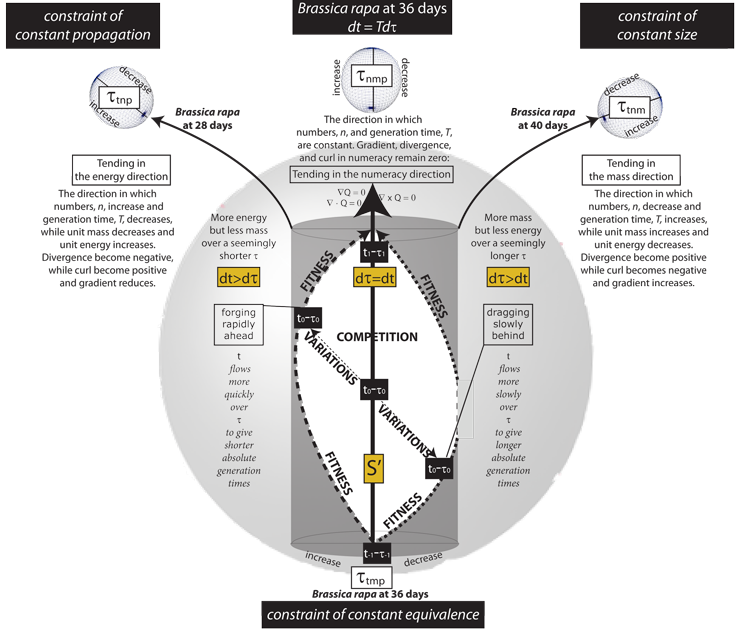
VI.2.1 The next set of rules are the four maxims of ecology. They establish the path-connectedness of the X⁄~ and Y⁄~ identification spaces … and therefore their homeomorphism. They govern the meridians that create the divergences and curls through the spherindrical τt, τn, τm, and τp diameters and their bounding cubinders. Figure 40 does its best to represent their various four-dimensional relationships, taking Brassica rapa as a test case.

VI.2.5 The two sides of the equators on all the glomes are created by different Möbius strip activities. They therefore have different processing rates. One side accelerates above S’, the other decreases below it.

VI.2.6 Figure 40’s very large τtmp glome has been flattened by the τn hyperplane. It is therefore without number. Its large black central arrow is its spherindrical diameter. It establishes the per entity processing requests that carry the population straight towards the small τnmp numeracy glome at top and centre.

VI.2.7 The small τnmp numeracy glome at top and centre has been flattened by the τt hyperplane. It therefore receives all momentums, and governs all emergent surfaces. Since it is without t, it must follow the second law of thermodynamics. Its values therefore fly away into the surroundings. It guarantees that every population will dissipate. It states the S = (n, m̅, p̅) activity rate for an entire population. It sets the equilibrium population numbers observed as the numeracy, Q, over each circulation distance, dτ, and each time interval, dt. It is rectilinear. It is the only one observed.

VI.2.8 There is no shorter route about our four-dimensional S3–V4 τtnmp rotachoron than the τtmp glome’s large black arrow. It goes straight to the τnmp glome. It punches directly from τ-1t-1 at the beginning of a generation, to τ1t1 at the end. Any population following it travels on all four equators, simultaneously, and is immediately following that shortest of all possible paths. It is the cubinder that provides the identification space’s equilibrium rates. We measured it, for Brassica rapa, at T ’ = 36 days.

VI.2.9 The τtmp and τnmp glomes also establish the identification space’s “temporal divergence”. This is the characteristic set of equilibrium biological processing requests made per each unit of time across that population. It helps create both the stasis of the first kind of ∇Q = 0, and the ∫dS = 0 constraint of constant equivalence. This overall temporal divergence is coordinated through dt = Tdτ and dS’ = dn’ + dm̅’ + dp̅’.

VI.2.10 Both the dt = Tdτ and dS’ = dn’ + dm̅’ + dp̅’ that determine population behaviours in any identification space are suggested rates. Neither fixes an invariant absolute time interval.

VI.2.11 Our Brassica rapa experiment measured the two linespaces to right and to left as T = 40 and T = 28 days respectively. Both are longer than the central T’ = 36 day path. They affect τ and T differently across the four dimensions. They are each longer in different ways.

VI.2.12 The τtnm glome at top right has been flattened by the τp hyperplane. It therefore sets the identification space’s nucleotide chemical component flux as the ∫dM = 0 constraint of constant size.

VI.2.13 When the population selects its 40-day path and heads towards the τtnm population components flux glome, then it is leaving the S’ that is both the Möbius strip contact point and the equator. It moves to the sides of all three other glomes. There will be linked changes in those other rates.

VI.2.14 Since dS’ = dn’ + dm̅’ + dp̅’, then the Brassica rapa population cannot move to the side of one glome without moving to the opposite side of at least one other. For every ipsilateral movement at one place and time, there is a contralateral one.

VI.2.15 We look first at the ipsilateral movements. When Brassica rapa selects the path to the right of the small τtnm glome, it also selects a path to the right of the large τtmp one. This dτ extends the total number of biological processing requests made to the population. It therefore extends in τt, which is to increase the temporal divergence.

VI.2.16 The ipsilaterality exhibited by the small τtmp glome at the right is the increased temporal divergence. It is the increase in the overall processing orders given to the population at each point about the circulation. It undertakes an increased amount of biological processing. This is dτ > dt.

VI.2.17 But that increase in biological processing demands is made without an accompanying increase in the rate at which the orders can be fulfilled. So with that dτ acceleration in processing requests comes a necessary increase in the absolute time, T, the population will need for all that extra processing.

VI.2.18 As in Figures 35b and c, the time each individual entity must now allot to the extra processing extends the overall circulation length. The Brassica rapa generation length therefore extends to T = 40 days.

VI.2.19 The path to the right of the τtnm glome again increases m̅. This increases the average number of chemical components held per entity. This further increases the total requests made to the population. But there is again no immediate accompanying increase in rate of working. And further since the amounts entering each individual entity increase, the population mass flux, M, increases. The divergence in the mass flux is therefore given by ∇ • M = m̅.

VI.2.20 However, every circulation in a biological and Hausdorff identification space that has an ipsilateral increase requires some countervailing and contralateral decrease. A positive transition in the small τtnm, and in the large τtmp, glomes must be accompanied by corresponding decreases upon the two small τtnp and τnmp glomes at centre and at left, which must therefore have negative divergences.

VI.2.21 The τtnp glome at top left is flattened by the m hyperplane. It therefore sets the population’s unit energy density. And since it is contralateral, a move to its right is a reduction. This decreases the unit energy made available to fulfill the increased requests made, at each clock moment t, through the large τtmp glome. The absolute time, T, required must therefore increase. This is again the 40-day Brassica rapa path.

VI.2.22 And then additionally, a move to the right of the τnmp numeracy glome, at top centre, reduces the population density, N. The absolute numbers, n, in each time interval, dt, must therefore decrease.

VI.2.23 Since these are four-dimensional interactions, then the combination of these various ipsi- and contralateral glome transitions means that the dS’ = dn’ + dm̅’ + dp̅’ equilibrium increases m̅, increases T, decreases n , and decreases p̅.

VI.2.24 The small τtnm glome on the right therefore uses its coordinated γ activities to oversee the overall Ingredients 4 replacement. One side of its equator increases the divergence in the population mass flux of chemical components as +γ = +(∇ • M) = +dm̅’; while the other decreases it as -γ = -(∇ • M) = -dm̅’.

VI.2.25 The zero divergence at the τtnm glome equator is the population’s equilibrium S’. That value pervades the entire identification space and establishes the m̅ for the plesseomes characteristic of the plessemorph in any population.

VI.2.26 Since Brassica rapa’s 40-day linespace to the right favours the τtnm glome, it increases population entity masses. But it simultaneously raises the number of processing requests imposed upon them via the large τtmp glome; while disfavouring (a) the energy intensity; and (b) the population numbers that can achieve this. It reduces these through the τtnp and τnmp glomes at left and centre.

VI.2.27 And since the path to the right is longer, it moves the population to the outside of Figure 9’s helicoid track. And further since that longer path has an overall reduced work rate, then it takes longer to traverse.

VI.2.28 And … we indeed observed, in our Brassica rapa experiment, that this path had a reduced pot density of only four plants per pot; but the plants had increased masses; along with an increased generation time. And since that small τtnm glome to the right oversees those Ingredients 4 γ replacements in λ, then its net behaviour governs:

Maxim 1: The maxim of dissipation [Darwin’s theory of competition]

∫dm < 0; ∇ • M → S’; M = nm̅.

(A) Any entity that can lift a weight will be prevented from so doing; and/or (B) can be put to use for the same purpose. (C) No entity can lift a weight indefinitely.

VI.2.29 Any Brassica rapa linespace that leaves the S3–V4 rotachoron equator automatically creates a longer circulation. Therefore, even though the linespace heading towards the small τtnp glome to the left has T = 28 days and so is shorter in time, it must be longer in some complementary way.

VI.2.30 The path to the left moves to the left of the τtnp energy activity glome. It must therefore increase the population’s unit energy density … which is to increase its rate of activity, p̅

VI.2.31 But this path is contralateral with respect to the previous two glomes: the small τtnm and large τtmp ones. The former must now decrease the divergence in the mass flux. This makes entities smaller by reducing m̅. The latter must decrease the temporal divergence by reducing the number of biological processing requests made, which is dt > dτ.

VI.2.32 This path to the left of τtmp therefore imposes a decreased demand for biological processing about the circulation. But the τtnp energy glome’s own movements simultaneously increases the population’s energy capability. This allows the population to move to the inside of the helicoid, which is the shorter track. The increased activity rate means that even though this path is longer, it takes less time. We observed this, in our experiment, as that T = 28 days.

VI.2.33 But there is also an ipsilateral shift to the left of the τnmp numeracy glome. This is an increase in number density, N. We observed the increased path length as an increase in pot density to fourteen seeds per pot.

VI.2.34 We have here an increase in the lengths over two dimensions. They favour the τtnp glome by increasing the divergence in the energy flux, ∇ • P, which is by increasing p̅; but they also increase the divergence in N. We may again be travelling about a longer path, but we do so much more quickly.

VI.2.35 The τtnp glome to the left governs the Ingredient 3 ψ chemical bond energy flux, dp̅, for the plemes and plessetopes. Its equator establishes the plessemorph energy throughout the identification space. The glome is therefore:

Maxim 2: The maxim of number

∇ • P = P⁄n = p̅

The number of progeny produced depends upon the number of progenitors maintained.

Figure 41: Divergence and curl

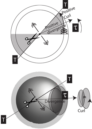
VI.2.36 Every curved line, every rotagon, every rotahedron, and every rotachoron is created by snipping some Möbius strip object. More generally, and as in Figure 41, any V2 biovolume such as an A = πr2 is accompanied by the one-dimensional measures r and c = 2πr. If the area changes then r also changes. But since this is T = 2r then dt is non-zero, and the curl also changes.

VI.2.40 But population numbers simultaneously have a contralateral decrease about the τnmp numeracy glome. That net change is the partial derivative -∂n⁄∂t.

VI.2.41 Since M = nm̅; and since the population’s mass flux, M, occurs over the entire interval T; then the total over the entire generation is ∫M dT.

VI.2.42 However, each individual entity has a mass, m, at every point. If their number is n, then their average at every point is m̅. Since we now have both the numbers and their contributions at each point, then the total over the above interval is also ∫dm̅ dn.

VI.2.43 If the numbers remain constant over any T, then the net contribution each entity makes at each point, which is a charateristic for the generation, can be determined from ∫M dT = ∫dm̅ dn. Every entity that participates has this same value m̅’.

VI.2.44 However, if numbers change, then the characteristic contribution changes. It is no longer shared by all. The range difference is the curl in the mass flux. It is given by ∇ × M = ∫M dT⁄∫dm̅ dn.

VI.2.45 Brassica rapa’s slow 40-day path sees such a large +∂m̅⁄∂t that the characteristic increase in masses over the remaining members more than compensates for the decreased numbers, -∂n⁄∂t.

And similarly, the faster 28-day path sees a decrease in the individual chemical components stock of -∂m̅⁄∂t. But that characteristic mass decrease is offset by a large increase in population numbers, +∂n⁄∂t.

VI.2.46 The net result, over Brassica rapa’s identification space, is that, in the first place, populations on the helicoid’s inside 28-day pole position track have increased numbers, and work at a faster rate. They contribute to the identifcation space by using their increased curl in numbers, +∂n⁄∂t, to compensate for their reduced divergence in mass, -dm̅.

But in the second place, plants on the slower outside 40-day track work at a slower rate. They contribute to the same identification space by using their increased curl in mass, +∂m̅⁄∂t, to compensate for their reduced divergence in numeracy, -dQ.

VI.2.47 Whenever population numbers, n, in any X⁄~ or Y⁄~ identification space change, then there is a curl in mass of ∇ × M = ∫M dT⁄∫dm̅ dn. The contralateral and countervailing changes in n and m̅ allow the population to balance its two sets of divergences and curls in mass and in numeracy. The net change in the chemical components flux, M, is given by:

Maxim 3: The maxim of succession [Darwin’s theory of evolution]

∇ × M = ∂m̅ ⁄∂t - ∂n⁄∂t

The rate at which progeny is produced depends upon the rate at which competition occurs.

VI.2.48 Energy density changes are the most variable. There can be population wide changes in p even as both m and n remain constant. But both M = nm̅ and P = np̅ always exist. Since n = M⁄m̅ = P⁄p̅, then there must be a work rate, W, upon any path, and such that W = m̅⁄p̅.

VI.2.49 The divergence in numeracy is ∇ • Q = m̅final - (m̅initialninitial ⁄nfinal). The divergence in the chemical components flux is ∇ • M = m̅. The mass flux can change with no effect on numbers, but the numbers cannot change without affecting the curl in the mass flux, ∇ × M.

VI.2.50 The curl in numeracy is ∇ × Q = p̅finalm̅initial(nfinal - ninitial). It can only remain zero if n does not change when M changes. But this then means that the population is pursuing the shortest possible path. It is following the cubinder that is the large black arrow, for the equatorial path, and so is heading straight towards the τnmp glome.

VI.2.51 If numbers stay the same over T, then each entity’s net and characteristic contribution to the population energy flux over the generation, p̅’, can be determined from ∫P dT = ∫dp̅ dn.

VI.2.52 The path that holds n constant by ensuring that M and P change at the same rates as m and p, is the cubindrical one that surmounts the equator. It sets W = M⁄P = m̅⁄p̅. All other paths are longer due to their curls in both mass and energy … and as caused by the resulting curl in number.

VI.2.53 Since P = np̅, then only a set of inverse changes in n and p can link the divergence to the curl. The curl in energy of ∫P dT⁄∫dp̅ dn is driven by ±∂dp̅⁄∂t and ±∂n⁄∂t.

VI.2.54 The Brassica rapa linespace to the left is longer because even though plant masses decrease, numbers and energy density both increase. This increases the work rate, W, through a curl given by the partial differential ±∂W⁄∂t. The path is then travelled more quickly.

VI.2.55 If our plessists and/or plessemorphs are to create paths within the identification space that allow for the required ipsi- and contralateral accelerations and decelerations that preserve the species equilibrium of S ’ = (n’, m̅’, p̅’), then there must be a curl in energy involving all three properties ∂p̅⁄∂t, ∂W⁄∂t, and ∂n⁄∂t as:

Maxim 4: The maxim of apportionment

∇ × P = ∂p̅⁄∂t + ∂W⁄∂t - ∂n⁄∂t

The bioactivity of a biological population is subject to increase from an initial value for one or more of three reasons: (a) increases in mass; (b) decreases in competition. All other increases are due to (c) the essential development of the entity or species.

VI.3.1 Our homomorphic structures can create all biology and ecology by linking to homeomorphic spaces through the three constraints and the three stases, thus defining the deformation retracts, S’, the mapping cylinders, Mλ, and the universal covering spaces, C, that are the size and properties for each X⁄~ and Y⁄~ identification space. And since each one’s structural equivalence is p ∼ q, where (p, ±q) and so that p = ±q, then any φ(U(X)) that selects any p in X has an open equivalence class φ-1(U(X)) that takes the whole of Y for its V(Y) to select ±q. And similarly, any φ(U(Y)) that selects any p in Y has an open equivalence class φ-1(U(Y)) that reciprocally takes the whole of X for its V(X) to select its ±q. Therefore the base B = BXY ∪ BYX is always the whole of both the progenitor domain as preimage, X, and progenitor codomain as image, Y. The intersection BXY ∩ BYX always holds some path that describes some state, S, at every point in the generation, τ, and so that our four maxims of ecology define the fluxes that suitably pervade those X⁄~ and Y⁄~ identification spaces as the homeomorphisms that preserve the connected paths. We must now declare the four laws of biology that command the homomorphic structures and biological entities to actually follow those homeomorphic paths.

VI.3.2 The upcoming laws of biology must make definite statements about plessists’ and plessemorphs’ real-world behaviours so they follow the identification space’s homeomorphic paths.

VI.3.3 Although all individual members in any given population must ultimately dissipate, then by Meme 121 all populations must—as a whole—preserve both their homo- and their homeomorphisms by preserving the path-connectedness that guarantees homeomorphism. The n plessists and plessemorphs concerned must therefore follow whatever paths preserve BXY ∩ BYX and B = BXY ∪ BYX. They must in other words ensure that m̅ > 0 so the base always exists throughout the identification space.

VI.3.4 Although each distinct entity must again individually dissipate, each also participates in a population-wide system that must at some time exhibit the dm̅⁄dt > 0 and ∂m̅⁄∂t > 0 that maintain the number of their connected paths.

VI.3.5 But we can take any universal covering space, C, and form its identification space, C⁄η. We simply take any point p, up in the cover, and then deformation retract it to some single point. We then use the same p = ±q equivalence to create a structural p ≈ q equivalence over the remainder.

But the C⁄η identification space, up in the cover, is the not-p that surjectively covers the entirety of the base space, B. Therefore, and as in Figure 7, every point in the base is accessible from the universal covering space’s real projective plane and identified points. As in Figure 32, we now have an extant Möbius strip between cover and base, and between base and cover, with s ◦ s’ = τ and s ◦ s-1 = S’, and through which the two can reciprocally access each other, all across the generation, as progenitor domain and preimage, X, and progeny codomain and image, Y.

VI.3.6 Every population resides on a real projective plane and expresses its transformations in homogeneous coordinates. Although Maxim 1 insists that all entities must eventually dissipate, it also guarantees that at least some members will curl to the right-hand side of the τtnm glome. They exhibit a positive divergence in the mass flux, M. Those members follow paths that take them to the projective plane’s identified edges. They therefore have m → ∞.

VI.3.7 By Meme 96 and Meme 99 some determinable period T exists so that ∫dm ≥ 0 and ∫dp  ≥ 0 is always true over a sufficiently large enough number of entities. And since all viable populations must preserve both homo- and homeomorphisms, then there must always be at least one member in any X⁄~, Y⁄~, and C⁄η identification space that preserves those path connections. We must always therefore have n ≥ 1.

VI.3.8 By Meme 122, when all members in all populations follow ∫dm < 0 and ∫dp < 0 and succumb to Maxim 1 of dissipation, they also flatten with the τt hyperplane. They head towards the τnmp numeracy glome. This creates all a population’s observable real-world values of n, m, and p at each moment t. All distinct biological entities must, in other words, follow the second law of thermodynamics. They must increase in their entropy. However, if the population is to be preserved, then each population must persuade at least some of its entities to follow the doctrine of “negative entropy” first proposed by Erwin Schrdinger (Schrdinger 1944). This is the combined effect of the glome equators, and their S’ Möbius strip crossing point.

VI.3.9 The effect of Schrdinger’s negative entropy on paths and identification spaces is that if a given population is to reproduce, then both its progenitor domain X as preimage and its progeny codomain Y as image must always have open, non-empty, and Hausdorff sets. Each must access a U within itself and a V within the other. All intersections of all these Us and Vs, BXY ∩ BYX , must be non-empty. They must always produce the base B = BXY ∪ BYX. The identifcation spaces X⁄~, Y⁄~, and C⁄η must not simply exist. They must be followed.

VI.3.10 But since all entities must eventually dissipate, then the number of disconnected and empty paths in any X × Y product space greatly outnumbers the number of connected ones. There is then no homeomorphism, no replication, and no species. Therefore, the paths that any current entities in any X and Y follow can easily make B = BXY ∪ BYX non-existent, so that BXY ∩ BYX is empty and there are no viable extant entities.

VI.3.11 A viable biological system must therefore lift new and connected paths into itself to replace all disconnected ones lost by its non-viable and/or dissipating members. The homomorphic and homotopically equivalent members must act as bases; as fibres; and as fibre bundles. They must reconstruct all disconnected paths.

VI.3.12 Our plessists and plessemorphs, as biological entities, must configure their countable Ingredient 4 atoms so they maintain a constant material presence throughout the entirety of the identification space. They must constantly use γ and ψ to maintain Schrdinger’s negative entropy, meaning they must always do work, W, as clearly defined by the first law of thermodynamics, and so that: δW = (δQ - dU) > 0 (Encyclopaedia Britannica 2002).

VI.3.13 Every viable population that wishes to preserve paths must abide by both the constraint of constant size of ∫dM = 0 and the stasis of the second kind of ∇ • Q = m̅final - (m̅initialninitial ⁄nfinal). Both (a) the homomorphic members, and (b) the molecules they use to compose themselves must be equipollent with ℵ0 (Weisstein 2015a). All the above requirements, taken together, give:

Law 1: The law of existence

n > 1; δW = (δQ - dU) > 0; m → ∞; m̅ > 0.

There is an entity such that it must always lift a weight; and such that it must, and by this means, at some time increase in its mass.

VI.3.14 Not only must the equivalence classes defined by the X⁄~, Y⁄~, and C⁄η identifcation spaces always exist, but they must have a structural and measurable form. The X⁄~ is the entire Y codomain of progeny all across the generation, and as viewed by any progenitors at any time, t; while the Y⁄~ is the entire X domain of progenitors as again viewed at any time by any progeny; with C⁄η then being an entire generation’s worth of both, and as viewed at any time from any point in the universal cover … which is then also the entirety of the mapping cylinder, Mλ. But that is itself γ and ψ combining as the fibration and cofibration that are the entirety of any given biological–ecological activities, λ.

VI.3.15 If the homomorphic structures are going to reproduce, then they must follow the homeomorphic paths the identification space makes available. They must be constant topological neighbours all about Boy’s surface and so must constantly share the same positive and negative absolute values and rates of change. But since the universal covering space, C, is also the mapping cylinder, Mλ, then this has very particular consequences.

VI.3.16 Our homomorphic structures must be constant topological neighbours throughout their X⁄~, Y⁄~, and C⁄η identification spaces. We can therefore note that in 1927 the English zoologist and animal ecologist Charles Elton proposed an identification space for all members of the same species as their shared set of behaviours in their equally shared surroundings:

It should be pretty clear by now that although the actual species of animals are different in different habitats, the ground plan of every animal community is much the same. In every community we should find herbivorous and carnivorous and scavenging animals. … It is therefore convenient to have some term to describe the status of an animal in its community, to indicate what it is doing and not merely what it looks like, and the term used is “niche”. Animals have all manner of external factors acting upon them—chemical, physical and biotic—and the “niche” of an animal means its place in the biotic environment, its relationship to its food and enemies. The ecologist should cultivate the habit of looking at animals from this point of view as well as from the ordinary standpoints of appearances, names, affinities, and past history. When an ecologist says “there goes a badger” he should include in his thoughts some definite idea of the animal’s place in the community to which it belongs, just as if he had said “there goes the vicar”. [emphasis in original] (Elton 1927).

VI.3.17 We have found our identification spaces. We have also found our equivalence classes.

VI.3.18 Let there now be a Population R; and also a Population S. If they are indeed members of the same species, then they will have the common base B. They will share:

• the fundamental group π(B);

• the constant loops α0 to F, which are equivalently α0 to α0, and/or F to F;

• and the transformations φ:X → Y and φ-1:X → Y, which latter is φ:Y → X.

VI.3.19 Since Populations R and S follow homeomorphic paths, then their X and Y subpopulations that are the progenitor domain and progeny codomain are also each others’ deformation retracts. Their entities will occupy neighbourhoods near to each other on both their mapping cylinders as Mλ(R) and Mλ(S); and their universal covering spaces as C(R) and C(S).

VI.3.20 If our Populations R and S are indeed members of the same species then as Rossberg et al point out, their subpopulations R(X), R(Y), S(X), and S(Y) must be more than merely homomorphic and homotopically equivalent:

The niche concept has remained of fundamental importance to ecology. It establishes a link between individual-level traits and population dynamics. … The availability of an ecological niche for a species depends, in a great variety of ways, on interactions between the species comprising an ecological community. These interactions, in turn, are affected by the phenotypic traits expressed in the interacting species. … However, despite decades of intense research and debate no universal agreement has emerged as to how niches are to be formally represented, and fundamental questions remain unresolved (Rossberg et al, 2010).

VI.3.21 We can easily correct the deficiency Rossberg et al highlight. As we saw with the letters X and Y, homomorphic objects can lose information when mapped to each other. The four-to three-vertex φ:X → Y mapping is not the same as the three- to four-vertex φ:Y → X. These are not bijective. They do not have the same underlying structure.

The mappings φ:R(X) ↔ S(X) and φ:R(Y) ↔ S(Y) between populations that successfully reproduce are, however, invertible. They are homomorphisms possessing both the φ and φ-1 mappings. They are therefore isomorphic.

An isomorphism is a homomorphism between any two sets or structures that have a one-to-one correspondence between their elements so their group operation can be reversed. The bijective mapping means the objects have the same underlying structure, and must also be homeomorphic.

VI.3.22 The isomorphic Populations R and S now share a joint base, B. They interact with a shared universal covering space, C. Every point x in B has an open neighbourhood U(X). Their shared mapping, ξ, projects—with Mbius strip—from cover down to base. The inverse ξ-1 mapping of the fibre from base back to universal cover is the lifting of the disjoint union of open sets, ξ-1U(X), into C, and again with Mbius strip. Those then avail themselves of the same Mbius strip to immediately map surjectively, and homeomorphically, back down onto U(X) with ξ.

VI.3.23 Since Populations R and S are biological, their open sets are their progenitor domain, X, and progeny codomain, Y. They are therefore isomorphic across their respective circulations of the generations, τ.

VI.3.24 Since the universal covering space, C, is topological, it has its own fundamental group. This must be surjective, , over the base fundamental group, π(B) … which is immediately injective, , back into the cover’s.

VI.3.25 Since π(B) is injective into the universal cover, then for every path starting at the base’s x0 identity, there exists a path up in the cover beginning at the cover’s identity. So once we fix any loop start point α0 in the base, we fix a corresponding start point in the cover. Every loop in the base, as a preimage, has a unique image in the cover. If, therefore, Populations R and S are isomorphic in the base, they remain isomorphic when lifted to the universal covering space, C.

VI.3.26 A deck transformation, η, is an isomorphism from a covering space onto itself.

VI.3.27 Any given deck transformation, η, is completely determined by whatever point upon it the fibre lifting into it accesses. Both η and any φ:X → Y and/or φ:Y → X remain unchanged and unique.

VI.3.28 If a first universal cover, C(M), projects an ξM down into some base, B; and if a second universal cover, C(N), sends its ξN down into the same base; then C(M) and C(N) create the same surjective mapping, and must receive the same injection from B. Each will therefore be carried from and to the same places in B. And since they achieve the identical effect, no matter what injective ξ-1(U) fibre they each receive, then C(M) and C(N) are isomorphic.

VI.3.29 The C(M) and C(N) universal covering spaces share the identity property η ◦ φ = φ ◦ η = φ, and have the effect ξM = ξM ◦ η = η ◦ ξM = ξN ◦ η = η ◦ ξN = ξN. Their deck transformations η:C(M) → C(N) and/or η:C(N) → C(M) are therefore also bijective.

VI.3.30 For any loop from any α0 in the base B; and for its matching universal cover transformation; then the π(B) fundamental group acts by deck transformation to create unique points up in the cover.

VI.3.31 Since Populations R and S will also interact with the surroundings as a mapping cylinder, Mλ, then again as in Figure 7, they have both a fibration and a cofibration. Their cofibration, ρ, lifts from their progenitor domain as preimage, X. It is isomorphic with the surjective projection, ξ, coming down from the universal cover into the base. And their fibration, q, lifts from the progeny codomain as image, Y, and is isomorphic with the injective ξ-1 lifting from base back to universal cover.

VI.3.32 Since those of our homomorphic structures that exhibit both the sets of transformations φ:X → Y and φ:Y → X are invertible, then they are isomorphic. They are therefore bijective. And those that are indeed bijective can freely exploit the invertible paths in our homeomorphic identification spaces X⁄~, Y⁄~, and C⁄η.

VI.3.33 Our isomorphic structures therefore correct the deficiency in Elton’s ecological niches that Rossberg et al highlighted:

• They can follow connected paths that undertake all biological ρ and cofibration activities. They can abide by Law 1 and do work as, for example, sperm that swim to fertilize; eggs that polarize; fruits that discard their husks while their endosperms germinate their seeds; and etc. These seemingly negative entropy—but work-preserving—paths lift masses, energies, and heat into the surroundings as -γ and -ψ.

• The isomorphic and so invertible structures that are the resulting progeny can then also follow connected paths. They undertake such θ fibration and biological activities as grazing, browsing, photosynthesising and the like. These all also abide by Law 1. They require work and emit heat … but they instead lift masses, energies, and heat from the surroundings back into the population as +γ and +ψ.

The former set of activities are -l and take place through -r. They send about one loop in a Whitney umbrella, as -dA and +dA, out and back to V0. The latter are +λ, taking place through +r, sending about the other loop as +dA and -dA, to and from the same V0. The former emit through the population’s S0 outputs as -γ and -ψ; while the latter absorb through the S0 inputs as +γ and +ψ. The S0– V0 are together the set of biological-ecological activities, λ.

VI.3.34 We have successfully defined our π≡ [(1 × 1δ=1 → 1)1 ⇔ (1 ÷ 1δ=1 → 1)1] equilibrium. It characterizes our X⁄~, Y⁄~, and C⁄η identification space. It declares that if our population wishes to maintain a characteristic equilibrium over a given set of entities, then (a) they must have isomorphic biological structures; and (b) they must occupy homeomorphic spaces. Only then can they cross a real projective plane so they equalize their inexact differentials of their gradients, divergences, and curls with the exact differentials of their three constraints. The entities concerned will then move constantly through each others’ neighbourhoods over both a shared circulation length for a Mbius strip, τ, that is both sides of Boy’s surface; also doing so in the same absolute time interval, T.

VI.3.35 The above isomorphisms and their accompanying homeomorphisms for a given identification space provide:

Law 2: The law of equivalence

[(δW1 = δW2) ^ (δW2 = δW3)] ⇒ (δW1 = δW3)

If a first entity can follow a path such that Law 1 is satisfied; and if a second entity can follow the same path to the same effect; then the first and second entities are equivalent.

VI.3.36 Both our rotachoron and our real projective plane are four-dimensional, with the former’s equator being the latter’s snipped Möbius strip crossing point. And since the real projective plane uses homogeneous coordinates, then all points on apparently opposite sides of any equatorial line or surface are identified.

VI.3.37 By Law 2, our new law of equivalence, every viable population has its X⁄~, Y⁄~, and C⁄η identification spaces that state its specific p = ±q equivalence classes. And by Meme 123, we can identify all species via their [Σ = {A, C, G, T}, S = {n, m̅, p̅}, δ, α0, F] Chomsky production rule which sets δ to some value that establishes both their initial and their final biovolumes, V1,2,3,4, and accompanying biosurfaces S0,1,2,3.

VI.3.38 By Meme 124, those same Chomsky productions operate over a base, B, that is a set of both progenitors, X, and progeny, Y, that interact over a circulation length, τ, for the absolute time period, T. They can maintain their Law 2 equivalence by lifting, and so injecting, their disjoint and open sets ξ-1U(X), as fibre, into their universal covering space, C. And no matter how much the base transforms its progenitors and/or progeny, the deck projects them straight back down. It always has ξ ◦ ξ-1 = # = τ = S’. The same overall state is restored about a Möbius strip that has that given crossing point, and is of that given length.

VI.3.39 Given the above, then there is also always a one-to-one mapping between the universal covering space’s deck transformations, η, and the base’s fundamental group, π(B).

VI.3.40 Since deck transformations are fully homeomorphic with the base fundamental group, then every constant loop s ◦ s-1 in the base has an initial point, α0, that is also some definite point, A, in the universal cover. And as the base loops towards its final point, F, then so also does the deck tend towards its own termination point. The base’s loop, with its inexact differentials therefore matches the deck transformations, with their exact differentials.

VI.3.41 But although our base has isomorphic structures that can follow homeomorphic paths, it also has very many more dissipative ones. We cannot yet isolate the isomorphic from the more generally homomorphic. Even though only isomorphic structures can preserve homeomorphism, any inexact differentials emerging from homomorphic—and therefore merely homotopically equivalent—structures, as say δFh, are presently non-different from the δFi inexact differentials that emerge from our isomorphic ones. The latter differ, however, by being equivalent to the cover’s exact differentials. The δFi therefore preserve path-connectedness, while the δFh do not.

We must distinguish the isomorphic φ(U(X)) subpopulations in X that can produce the δFi inexact differentials. These can form the V(Y) in Y that are also the φ-1(U(X)). Those V(Y) in their turn become the φ-1(U(Y)) that can use some complementary δFi to produce a V(X) that is once again a φ(U(X)). The U(X), V(X), U(Y) and V(Y) subpopulations and their inexact differentials must therefore share an identity so that any φ(U(X)) can beget a further such set that can in its turn preserve that same X⁄~, Y⁄~, and C⁄η identification space where B = BXY ∪ BYX, and where BXY ∩ BYX is non-empty.

VI.3.42 The heart of the replication enshrined in our π≡ [(1 × 1δ=1 → 1)1 ⇔ (1 ÷ 1δ=1 → 1)1] equilibrium Hooke cell and its Whitney umbrella is precisely this equivalence between its exact and its inexact differentials. We must state the relevant inexact δF increment in terms of some exact one. This requires an identity operation over both the exact and the inexact.

VI.3.43 At its most simple, the integral calculus tells us the magnitudes of any changes; while the differential calculus tells us their rates. Euler understood clearly that an identity operation leaves things unchanged, so that x + 0 = x, y × 1 = y, z - w + w = z, and p × 1⁄q × q = p. He realized that an integral exists that is its own derivative, so that the curve ex has the rate of change x. The identity operation leaves things unchanged for if we infinitesimally increment, or decrement, ex, we get ex.

We can now represent our δF inexact differential as the difference between two arbitrary functions G(x, y) and H(x, y) (Fitzpatrick, 2006b; Saad, 2007). If they are G(x, y)dx + H(x, y)dy, then their difference, as an inexact differential, lies in their two partial differentials, for ∂G/∂y ≠ ∂H/∂x.

There must, however, exist a solution, at some point, such that δF = Gdx + Hdy = 0. If we divide by Hdx, we can express dy/dx in terms of G and H. This gives dy/dx = -G⁄H = c.

We now have an entire family of curves, in the xy plane, with the same c. We can express that family as Γ(x, y) = c. We thus have the exact differential dΓ = (∂Γ/∂x) dx + (∂Γ/∂y) dy = 0.

If we now divide dΓ by dx, we will have a value for dy⁄dx. We get dΓ = (∂Γ/∂x) + (∂Γ/∂y) dy⁄dx = 0. But we have already determined that dy/dx is -G⁄H. We therefore have dΓ = (∂Γ/∂x) - (∂Γ/∂y) G⁄H = 0. Our original two inexact partial differentials now hold the exact Γ in common, so that H (∂Γ/∂x) = G (∂Γ/∂y). We can finally make our two partial differentials the independent variables in some further function, σ(x, y), so that (∂Γ/∂x) = σ(x, y)G and (∂Γ/∂y) = σ(x, y)H. We now have the exact expressions G = 1/σ (∂Γ/∂x) and H = 1/σ (∂Γ/∂y). We can therefore resolve any inexact differential using an “Euler multiplier” or “integrating factor”, based on e, and so that f1 (x) = f2’(x) = 1⁄f1’(f2(x)).

VI.3.44 And we need an exact differential. Thanks to the German physicist Hermann Ludwig Ferdinand von Helmholtz, every energy transaction has one. In his 1847 memoir On the Conservation of Force he recognized the many different forms of energy systems can contain. He generalized them all—including the thermal—as internal energy, U. Each system can thus contain many different kinds of energy, such as chemical, electrical, eletromagnetic, etc. Everything, however, has thermal energy. The exchange interactions that internal energy can undertake are the thermal interactions, δQ, usually called heat, that contribute to the amount of internal energy, U, any substance or system has. Heat is the tendency for the molecules to move, and so to interact, with all other forms of energy. Its manifestation of heat, δQ, is simply the tendency to interact, thermally. But its entirely internal changes are the infinitesimal change, dU. So each system can potentially match its exact internal changes in state to any inexact changes it induces externally. This will equate dU and δQ through some Euler multiplier.

VI.3.45 Helmholtz also pointed out that all matter participates in two critically different kinds of interactions. These are (A) their “required states”; and (B) their “allowed states”.

VI.3.46 The German physicist Rudolf Clausius next allied Helmholtz’s observations to Euler’s exact/inexact discovery. He therefore shows us a method.

VI.3.47 Clausius simply set the inexact differential of one function equal to the exact integral of another, calling that second equalizing function entropy. It is an Euler mutliplier. It is an identity operator. It makes all cycles the same, for they effectively undertake the same identity operation.

VI.3.48 Systems demonstrate their entropy similarities via their temperatures, T. Their similarity in temperature occurs independently of their sizes and their energy stocks.

VI.3.49 Entropy, S, has all the characteristics of a substance. It is quantitative. It changes all states by admixing with all substances.

Since entropy is substance-like, it flows across boundaries. It is distributed throughout all matter. It flows in and out of all substances and systems seeking to equalize them all in terms of their interactions with the surroundings, at a given rate, and for a given amount.

VI.3.50 Thanks to Clausius, any two systems working between the same two end points have identity operations over topological—and measurable—Eulerian cycles. Large systems can undertake a greater number of entropy changes, over their larger sizes, while still being identical to smaller ones. They simply go through a larger set of changes for they have greater rates and amounts in entropy. But any two cycles moving between the same two end points have exactly the same net interactions with the surroundings. They each preserve an identity.

VI.3.51 The second law of thermodynamics now establishes the general behaviour of all matter by distinguishing between Helmholtz’s allowed and required states. The number of microfluctuations allowed to a system may be considerable, but the Euler–Clausius identity tells us that each system jettisons its excess allowed states at a rate that depends upon its own size. That is its entropy.

The cosmos procures entropy from systems by putting them through thermal energy transactions. Those force the system to relinquish at least a portion of its thermal energy externally, as heat, δQ, through some internal and infinitesimal change in state, dU.

VI.3.52 By the second law of thermodynamics, every system transforms inexorably towards its required set of states. Those transformations are its interactions with the surroundings. They are governed by the thermal energy it can establish, due to its temperature, T. Those required rates and transactions are its “stable equilibrium state”.

VI.3.53 There is also a vital difference between the “work interactions” and the “nonwork interactions” involved in establishing a set of required states as a stable equilibrium one. Work interactions can achieve measurable mechanical effects, δW, in the surroundings. Nonwork interactions, δQ, cannot. But both are inexact differentials. They are both “path functions”.

VI.3.54 There is therefore a difference between allowed and required states, and between work and nonwork interactions … and so between allowed and required paths and interactions. Many transfers of thermal energy, δQ, can produce changes in state, dU, at some one given temperature, T. But many transfers of thermal energy, δQ, can also involve changes in temperature, dT. However, whether they do or do not produce work, δW; and whether they do or do not involve changes in temperature, dT; all transformations of allowed sets to produce the required ones of the stable equilibrium state involve changes in heat, δQ.

VI.3.55 Temperature, entropy, volume, and pressure are examples of attributes that describe a system’s current state. They can be assessed both before and after any interaction, whether work or nonwork. Their transformations reflect any internal changes in state between some initial state, S-1, and whatever may be the final state, S1. They are exact differentials. And since they reflect those changes in state, then they are “state functions”.

VI.3.56 Work and heat, as path functions, provide a contrast to state functions. Path functions describe the effects a system has in the surroundings, and as it transitions between its states, and so via its state functions, S-1 and S1.

The transitions a path effects as δW and δQ can only be observed when they exit systems; cross boundaries; and enter the surroundings. They are the path effects of the state transformations.

VI.3.57 But since the path functions of work and heat are inexact differentials, then they are each also partial differentials. We can therefore relate them to our state functions and our exact differentials using our Euler multiplier.

VI.3.58 More generally: if the numbers of constraints, b, placed about any energy stock, in some system, hold constant; if its amount of substance also holds constant at N moles; if its internal energy is U; and if its entropy is S; then its change in entropy, as its energy changes, in its transition away from its allowed sets and towards its required ones is the partial differential (∂S⁄∂U)N,β (Encyclopaedia Britannica 2002). This is its “escaping tendency”.

VI.3.59 Since every system has such an escaping tendency, the second law of thermodynamics uses it to establish their behaviour. All material systems again distinguish between their required and their allowed sets via their above escaping tendency.

VI.3.60 The removal of constraints from around any allowed set always increases the number of its accessible states.

VI.3.61 The exploring of those acquired sets, via the escaping tendency, then increases the entropy.

VI.3.62 And when the system explores any extra and recently acquired allowed states, they in their turn escape via the escaping tendency as either only heat, δQ = dU; or else some of the heat also diverts into the doing of some work, δQ = dU + δW. But whether as more heat and less work, or as more work and less heat, all transformations the system undertakes reflect the same two end points. Any system may freely pursue any combination of inexact paths, but their sum between those same two end states is always the same exact differential, dU. This is the first law of thermodynamics.

VI.3.63 If, now, some progenitor domain X contains some Subpopulation U(X) with a greater escaping tendency relative to some Subpopulation V(Y) located in some progeny codomain Y, then even though both have an escaping tendency, energy will leave U(X) and transfer over to V(Y). The excess states in U(X) transfer over to the colder, or smaller, or more more tightly configured V(Y). The molecules in U(X) transform more extensively, forcing V(Y) to alter its states and its molecular distributions.

VI.3.64 And … a lower escaping tendency is immediately a greater “capturing tendency”.

VI.3.65 Subpopulation V(Y) has a greater capturing tendency relative to Subpopulation U(X).

VI.3.66 Subpopulation U(X) is now changing in state. It is moving closer to the states exhibited by Subpopulation V(Y). But V(Y) is also changing in its state. It is transforming closer to U(X). They are both moving closer to a shared mean S’ maintained between them over time.

VI.3.67 All populations and systems with a greater escaping tendency now have a one-sided, and irreversible, effect upon all systems with a lower and escaping one. So if U(X) is larger, and/or located at (τ’t’ + x), then it changes in its state to become smaller and/or to be located at (τ’t’ - x). And if V(Y) is instead larger, and/or located at (τ’t’ + y), thenU(X) changes in state to become larger and/or to be located (τ’t’ - y) while V(Y) becomes smaller. They are as inverses tending to the same S’ at τ’t’.

VI.3.68 When the base, B, lifts and injects its disjoint and open sets into the universal covering space, C, as the ξ-1U(X) fibre, then the one-to-one mapping between its fundamental group, π(B), and the deck transformations, η, projects them straight back as ξ, and so surjectively onto U(X). And since all the final points, F, that the base injects into the cover are homeomorphic with that cover’s own terminal point, 0, then no matter what transactions the base undertakes, the cover maintains its path-connectedness. Its deck transformations, η, are unaffected, being maintained through ξ ◦ ξ-1 = # = τ.

VI.3.69 Since the universal covering space, C, is also a mapping cylinder, Mλ, then the base transformations must be isomorphic. All lifted paths are invertible. They preserve the cover’s homeomorphic paths … meaning they also preserve its deformation retract, S’cover..

VI.3.70 By Meme 125, our deck transformations, η—which (a) preserve the cover’s identity, and (b) are homoeomorphic with the base’s fundamental group transformations, π(B)—are path functions.

VI.3.71 When X ↔ Y so the progenitor domain X transforms into the progeny codomain, Y, which transforms back, then a set of base homomorphic structures has occuped a set of isomorphic states and pursued a set of homeomorphic paths. By Meme 126 those isomorphic fundamental group transformations, π(B), are state functions.

VI.3.72 Both the base and the universal covering space now contain both the inexact ∇Q = ∇ • Q = ∇ × Q = 0 and the exact ∫dP = ∫dM = ∫dS = 0 transformations. They are isomorphic in the former, and homeomorphic in the latter.

VI.3.73 The base begins at α0 and terminates in F. The cover begins at A and terminates in 0.

VI.3.74 The base and the cover must both begin in some initial state S-1 at τ-1t-1 and terminate in some final one S1 at τ1t1.

VI.3.75 Since the number of paths and states a population can explore before its identification space is disconnected is limited, then the η deck transformations have A → 0.

VI.3.76 But a population’s initial state S-1 at α0 in its base must also be inherited from its predecessors’ as their final state, F. Its own final state, S1, after completion of all its upcoming transformations, will have the measure, M. But its final and measured state M promptly becomes the initial state for its own progeny as their inherited F. And since the base’s isomorphisms match the cover’s homeomorphisms, then we have both A → 0 in the cover and F → M in the base.

VI.3.77 Since we have an isomorphism–homeomorphism coupling, then when the cover’s homeomorphic and surjective projection ξ arrives as an onto over the base’s U(X), then the base’s real projective plane forms the disjoint, open, and identified ξ-1U(X) fibre that sends isomorphically and injectively back to the cover. We therefore have a set of mutual progenitor domain and progeny codomain transformations as ξU(X) ◦ ξ-1U(X) = S’base.

VI.3.78 The points the base inject into the cover identify with the cover’s original projection to create the cover’s deformation retract as a set of transformations in the surroundings of ξ ◦ ξ-1 = S’cover.

VI.3.79 If some given group of entities is proposed as a species, then no matter how diverse those entities might be, they must be both isomorphic in the base and homeomorphic in the cover. They must construct both of our identities, being ξU(X) ◦ ξ-1U(X) = S’base, and ξ ◦ ξ-1 = S’cover. But these are both the central white line and axis upon the helicoid in Figure 9 … and a Möbius strip.

VI.3.80 By Law 1, at least some entities in every viable population must move to the right of their τtnm glome. But since the entities lie upon a real projective plane and are both isomorphic and homeomorphic, then they must move to the same glome’s left when lifted to the universal covering space. And since those are identified points, then they define its equator.

VI.3.81 The same holds for all four S3 glomes. They are the (τt, τn, τm, τp) V4 gongyl’s surfaces.

VI.3.82 Again by Meme 125 we can identify all species through their Chomsky production rule of [Σ={A, C, G, T}, S = {n, m̅, p̅}, δ, α0, F]. It incorporates δ.

VI.3.83 By Meme 126, we further identify the Chomsky production rule δ with the deck transformations, η, so that δ ≡ η. We therefore have δ = η = ξ ◦ ξ-1 = S’cover.

VI.3.84 By Meme 127, the Chomsky Cartesian product Σ × S must then be the ±dA that forms the Whitney umbrella loops. That same product is the X⁄~, Y⁄~ and C⁄η identification space.

VI.3.85 The Chomsky production rule, δ, that now states the deck transformations, η, establishes the biological language of biovolumes V1,2,3,4 and biosurfaces S0,1,2,3. And since these are configurations of nucleotide codons, then by Meme 127 their molecules and photons state all capturing and escaping tendencies.

VI.3.86 The deck transformations, η, can now push their capturing tendencies down into the base as both (a) a surjective ξ projection, and (b) a set of semantic V1,2,3,4 biovolumes. But since those capturing tendencies are simultaneously step-downs, then they are also the presenting S0,1,2,3 biosurfaces. And by Meme 111, then when they are pushed in the directions τt, τn, τm, and τp, they take the absolute clock times T, TN, TM and TP. to cover those respective circulation distances.

VI.3.87 The base can similarly lift its own capturing tendencies up into the universal covering space as both (a) an injective ξ-1 fibre, and (b) a set of syntactic S0,1,2,3 biosurfaces. They then act as traces pushed through hyperplanes to reconstruct the concentric n-spheres that are the biovolumes V1,2,3,4.

VI.3.88 The biological cycle is now a series of step-ups and step-downs between surfaces and volumes, and between base and universal covering space. As varied and distinct as they might be in each direction, when all four of the base’s inexact (τn, τm, τp)T , (τt, τm, τp)N, (τt, τn, τp)M, and (τt, τn, τm)P differentials are summed over all four directions, they are the cover’s exact (τt, τn, τm, τp) differential.

VI.3.89 Each of the four inexact differentials is a combination of divergences and curls:

• The (τn, τm, τp)T is the numeracy glome at top centre in Figure 40, varying all of n, m, and p between the minimum and maximum for the generation, with the T subscript meaning the temporal divergence holds constant so that the number of biological processing requests made per unit time is always dt = Tdτ.

• The (τt, τm, τp)N is the large glome that varies the biological processing requests, along with entity masses and energies over the generation, but with the divergence in numbers—which is the numeracy, Q—now holding constant.

• The (τt, τn, τp)M is the small glome at left that varies processing, population numbers, and energy density while the divergence in the population’s chemical components flux, M, holds constant, and quite irrespective of whatever population numbers are used to maintain them.

• And (τt, τn, τm)P is the small glome at top right that varies the processing, the population numbers, and the chemical components flux per each entity, with the divergence in the energy—and therefore the work rate—now holding constant.

VI.3.90 Each inexact differential also declares some value for entropy. The curl is both (a) a two-, and (b) a three-dimensional expression as work and heat in the surroundings. And since each divergence is a rate of change of some area, as ±dA, then isomorphism demands that any change in any divergence produces a curl; and that any change in any curl similarly produces a change in some divergence. The various values in n, m and p, at the different moments t about a circulation are linked via Figure 19c’s braid-3 of dS’ = dn’ + dm̅’ + dp̅’. The net changes in divergences and curls therefore incorporate all possible rates of change. They will always sum, across all four dimensions, to the exact differentials up in the cover.

VI.3.91 The changes in state that the inexact differentials impose can now distribute themselves freely over all possible paths in the base … but they will always sum together to the same value up in the cover.

VI.3.92 The biological cycle is now a set of loops and inexact differentials in the base, B, and a set of matching recursive functions and exact differentials in the universal covering space, C.

VI.3.93 The biological cycle is also a set of surfaces and volumes as syntaxes and semantics. The S0,1,2,3 syntaxes and the V1,2,3,4 semantics are matching and identified sets in both the base, B, and the universal covering space, C. The former are injective, the latter surjective. They are, furthermore, a combination of the required and the allowed sets maintained as a set of connected paths against the surroundings and as B = BXY ∪ BXY and BXY ∩ BXY. And since every volume has a surface, while every surface bounds some volume, then their biological language is the mapping cylinder of their joint deformation retracts, being S’base ◦ S’cover = S’.

VI.3.94 We now have, by Meme 128, the balance between the escaping and the capturing tendencies. That balance is a required set of S’ = (n’, m̅’, p̅’) as their mean, thereby creating the fibrations, θ, and cofibrations, ρ, that lift into the surroundings as the biological-ecological processes, λ. They are the γ and ψ interactions that are the plessist and plessemorph metabolism and phsyiology of the observed biological entities. This S’ is therefore the entities plus their ecological niche as the mapping cylinder, Mλ.

VI.3.95 By Memes 115 to 118, the universal covering space’s A → 0 semantics and the base’s F → M syntactics produce the isomorphic nonpollent, unipollent, pluripollent and totipollent structures via the joint homeomorphic surjective x projections, and the isomorphic injective x-1 fibre lifts … which are also the mapping cylinder q fibrations and r cofibrations.

VI.3.96 Since every x projection down from the cover involves Ingredients 3 and 4 in photons and molecules as a set of codons, then it is a gain in paths and in allowed sets within the base. It is therefore an equivalent transfer of entropy to the base. The entities now contain a capturing tendency.

Although the sum of the entropies as transferred between cover, base, and surroundings can never decrease, the projection from the cover to the base is promptly a net decline in the cover’s escaping tendency. It is a loss in its entropy, its paths, and in its allowed sets. And since the cover is the ecological niche, then it is a transfer to the entities.

VI.3.97 By the same token, every lift from the base into the cover is a gain in paths and in allowed sets within the cover, which is within the surroundings; but it is a loss in those same paths and allowed sets from the base … which is the entities as a set of progenitors and their progeny.

VI.3.98 The losses and the gains in entropy by the entities and the surroundings, and in their escaping and capturing tendencies are again equivalent.

VI.3.99 Since these transfers between base and universal covering space are equivalent losses and gains in DNA and proteins, then every population is defined by the spherindrical push that is its Mobius strip contact point, its rotachoron equator, and so the Σ × S Chomsky Cartesian product and identification spaces all across its specified generation length, T. These are all created by a specified and distinguishing set of DNA codons and proteins carried across the circulation. It is every population’s required set of S’ = (n’, m̅’, p̅’).

VI.3.100 All biological entities may now have a required set, as S’, but they must also have an allowed set of transactions. This is the Whitney umbrella’s loops and the helicoid steps and levels. It is the ±dS’ range over both (a) some circulation distance, and (b) some absolute time. These together are ±dτ–dt about τ’–t’.

That range is an expression of both (a) the stases of the first, second, and third kinds as the inexact differentials ∇Q = ∇ • Q = ∇ × Q = 0; and (b) the three constraints of propagation, size, and equivalence as the exact differentials ∫dP = ∫dM = ∫dS = 0. The population explores them as a set of isomorphic entities with a shared set of minima and maxima. Those are expressed in their ±λ, ±dλ, and ±d2λ activities in the surroundings, using the magnitudes and rates of change expressed through dτ⁄dt, d2τ⁄dt2, and d3τ⁄dt3.

The population’s Chomsky production rule of [Σ={A, C, G, T}, S = {n, m̅, p̅}, δ, α0, F] states their complete set of states as the dS’ = dn’ + dm̅’ + dp̅’ language of syntax and semantics all around S’. The various biosurfaces that are its S3 glomes, that present to the surroundings, move in their various directions as the spherinders and inexact differentials of (τt, τn, τm)P, (τt, τn, τp)M, (τt, τm, τp)N, and (τn, τm, τp)T. This produces their unique and exact (τt, τn, τm, τp) biological structures and behaviours as their diversity in states and paths around their S’ centre as their deformation retract. They move between their base, B, and their universal covering space, C, all across T. This is also their set of biological–ecological interactions, λ, with their mapping cylinder, Mλ, as a set of progenitors, X, and their progeny, Y, over both τ and T.

VI.3.101 Since everything occuring up in the cover—and so in the surroundings—about any circulation length, τ, for time T also occurs down in the base—and so within some specified entities—and conversely, then we now have the complete cycle of proteins and organisms in any population.

VI.3.102 Biological populations and entities are now similar when their boundary activities as (i) loops, (ii) syntaxes, (iii) semantics, and (iv) recursive functions are also similar. They express themselves in both the surroundings and a set of entities. They are isomorphic transformations along homeomorphic and identified paths. The range between minimum and maximum is the complete set of biological and ecological transactions, λ, across an entire generation, and is:

Law 3: The law of diversity

A → 0; F → M

The sum of all the paths that satisfy Law 2 constitutes the allowed set for the entity and its equivalents; while that which permits them to satisfy Law 1 constitutes the required set.

VI.3.103 The law of diversity states the overall set of connected paths that any X⁄~, Y⁄~, and C⁄η identification space must maintain. But the escaping tendency eventually forces all individual entities in any X × Y topology onto paths with no capturing tendency. Those are disconnected paths whose intersection, BXY ∩ BYX, is empty, falling outside the B = BXY ∪ BYX basis that links the progenitor domain X to the progeny codomain Y. The plessists dissipate via the τnmp glome, and are no longer isomorphic.

VI.3.104 If a population or species remains viable, then there has been a successful transmission of the necessary (∂S⁄∂U)N,β capturing tendency—and so hereditary information—between a set of progenitors and their progeny. That propagation of a discrete set of suitably configured chemical components from one material body to another produces, and requires, both energy and entropy. It services the capturing tendency that is constantly needed to offset the escaping tendency for the dissipation mandated by the surroundings as the second law of thermodynamics. This viability requires both (a) a syntax, and (b) a semantics; as also (c) a surface, and (d) a volume.

VI.3.105 If a population again remains viable, then some subset of of entities, ninitial, uses its capturing tendency to increase its internal energy by capturing a sufficient quantity of resources and energy from the surroundings. It donates at least a portion of those energies and resources, acting as progenitors, to some second subset, of size nfinal. That second subset must then exercise a similar and successive capturing tendency. This requires viable homeomorphic paths and isomorphic states.

VI.3.106 All groups and subgroups in any viable population must be homomorphic and homotopically equivalent, globally, or they are not biological. But since paths must always dissipate, then specifed subsets and subgroups must be both isomorphic and homoeomorphic, but can only be so locally. They establish the needed deck transformations up in the cover, and the π(B) fundamental groups in the base. The entities can then generate and regenerate each other using each others’ capturing tendencies. The given population has then maintained its global net balance in its capturing tendency with respect to the surroundings, by always again by acting locally.

VI.3.107 Every viable population that avoids extinction must maintain its global required set S’ = (n’, m̅’, p̅’), constantly using a local capturing tendency, (∂S⁄∂U)N,β, over the generation time, T, and circulation distance, τ. The latter’s inexact sums are included in the exact former.

VI.3.108 Since the Chomsky production production rule, δ, is both the mapping cylinder, Mλ, and the universal covering space, C, then every population is also a matched set of syntax and semantics, and surfaces and volumes as progenitors and their progeny. Each S = {n, m̅, p̅} is an expression of all start symbols, terminal symbols, and non-terminal symbols.

VI.3.109 Although the population must act globally to maintain a set of paths that are constantly homomorphic and homotopically equivalent, and so whose total capturing tendency over the entire circulation ensures a global isomorphism and a global homeomorphism … it is again not locally required of all entities, at all their local points, that they all be isomorphic. Paths are permitted to be locally Euclidean, and/or locally hyperspherical—which then support trivial cycles—without being locally identified with any opposite points. They need not individually and locally project to cross any real projective plane, although the plane exists, globally. It is, therefore, globally required that work be done over and above any required set to produce the increases in energy and resources that allow progeny to reproduce by increasing the net number of available paths and allowed sets … but this same need not hold at every local point.

VI.3.110 Not all fibre bundles must be locally trivial. Some are non-trivial.

VI.3.111 The three constraints of constant propagation, size, and equivalence, ∫dP = ∫dM = ∫dS = 0, first apply, and then remove, allowed sets. The stases of the first, second, and third kinds state are then the ranges that transfer those allowed sets between base, B, and universal covering space, C.

VI.3.112 Since the three stases are inexact, then not all entities that follow a biological path need follow a replicative one.

VI.3.113 Our recursive functions contain Möbius strip identifications, and thus produce the recursions that sustain a population. As in Figure 39, the biology globe is the set of activities on the increase side of the τtmp glome equator, the replication globe being those on its decrease side. They transmit themselves across our four-dimensional rotachoron and our real projective plane. They use the four different sets of transformation rules to recurve as the injective and the non-injective, the surjective and the non-surjective. They create all biology and fertility spaces and groupings which are the Chomsky hierarchy of nonpollent, unipollent, pluripollent, and totipollent that link base and cover.

VI.3.114 Just as the second law of thermodynamics requires that one—and only one—of the states allowed to a thermodynamic system be the stable equilibrium one; then so also is it required of any viable species that at the very least one—but allowably more than one—of the paths in its allowed set be such that BXY ∩ BYX be non-empty. This allowed set path then possesses all needed properties for U(X), U(Y), V(X) and V(Y), with U open in X, and V open in Y; and U open in Y, and V open in X. We then have B = BXY ∪ BYX.

And … that allowed set path is the path of reproduction. It evidences a decrease in both mass and entropy, but maintains the needed global π = [(x × 1δ → y)T1=1 ⇔ (y ÷ 1δ → x)T1=1] bijection between an identified X and Y, inexactly over four dimensions, and so as to make the resulting S’base equivalent to an exact S’cover, thus maintaining the combined deformation retract S’ and required set (n’, m̅’, p̅’). That allowed set path uses the capturing tendencies in both the base, B, and the universal covering space, C, to offset any sacrifices each is forced to make via its escaping tendency. Since this requires a constant input from and interaction with the Chomsky production rule and deck transformations, then both A > 0 and dA⁄dt > 0 must always hold. And since this allowed set path exists in any viable population, it is the path that passes to the τtnm glome’s left so that the population’s mass always remains greater than zero, but decreases overall, giving m̅ > 0 and dm̅⁄dt ≤ 0.

VI.3.115 This allowed set path maintains all biology and ecology. It is the one that crosses the real projective plane and creates all identified points. It maintains the base for all fibres and all activities ranging between a minimum and a maximum. It is a property of the entire population, and of the whole circulation of the generations. It creates a biological cycle when taken conjointly and globally. But it is not the property of either any one entity, nor of any one point, taken severally and locally. We therefore, and finally, have:

Law 4: The law of reproduction

[(dm̅⁄dt ≤ 0) ^ (m̅ > 0)] ⇒ [(dn⁄dt ≥ 0) ^ (dA⁄dt > 0)]

In the allowed set is at least one path such that mass is surrendered, and such that a further entity possessing the required set, and satisfying these four laws, results.