
Part III: Biological spacetime
III.1.1 We exchanged the temporality of a generation interface for the non-temporality of a biological–replicative one. But it is the absolute clock times, T, associated with the former that tell us the homomorphisms populations and their enities use to create their recurvatures. It is instead the manifolds, τ, associated with the non-temporal latter that tell us about the spaces and the homeomorphisms through which the populations and entities must transform. These are the surroundings.
Those various manifolds may be continuous and simply-connected, but we cannot assume that the plessists and plessemorphs as the set A, their plessiomes and plesseomes as the set B, and their plemes and plessetopes as the set C will create S-1 plessist populations, as (a-1, b-1, c-1) that will transform into S1 populations, as (a1, b1, c1), that will be both homeomorphic and homotopically equivalent, while their plessemorphs similarly transform from (aa, ba, ca) to (ab, bb, cb). The successors can easily disconnect from their predecessors so they have become either (a) completely nonbiological, or (b) members of alien species. Our Chomsky production rules do not yet guarantee orderly behaviour.
III.1.2 Since our manifolds can all be retractions, a first problem is that they can combine without necessarily sharing the same dimensionalities. Two very nearby locations can then have different effects. Whether as a single conjoined manifold or various separate ones, the joint manifolds creating any interaction as the fibration–cofibration at the replication point, or else as the biology–replication one that marks a generation’s beginning, will then have radically different consequences upon the same structures, simply through having different dimensionalities.
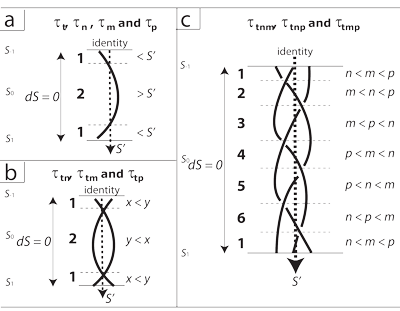
By Meme 80, the unknots and “one-braids” in Figure 19 represent the one-dimensional and one-manifold linespaces of τt, τn, τm, and τp. Just as do the gluing diagram in Figure 15c and the projective plane in 15e, they recognize that their two ends are continuous. If we glue those ends back together, we get the “closure of the braid” that restores each unknot. Each is then a continuous stream of homomorphic events that are certainly homotopically equivalent. When we, for example, combine t and n to make τtn, then the results in different places and times are most likely to be only homotopically equivalent. The two brought together can only be homeomorphic, given their different dimensionalities, if the locales always act in concert. So we must not only guarantee that each individual manifold can impose a recurvature on any given set of entities. We must also ensure that they keep behaving in the same ways when they interact.
III.1.3 If the population is to continue, then the wind walls must recurve. Each manifold must return to its beginning. We can distinguish between the homeomorphic and the merely homotopically equivalent, in such situations, by recognizing, for Meme 81, that each of our one-manifolds has three inter-related aspects:
• each recognizes the rectilinear ijk axes by overseeing a set of temporal sequences, dt, that create successive moments, t, across the absolute temporal interval 0 to T;
• each recognizes the curvilinear IJK axes by ranging from some minimum to some maximum, and back again, and so about its identity, S’;
• each recognizes the Frenet-Serrat TNB axes by transforming between Euler’s unit limits 0 and 1, and so by both the above infinitesimal increments dt and dS.
The total transformations that the radiating and circulating forces ψ and γ cause, across each manifold, and so from S-1 to S1, sum as ∫dS’ = 0. All unknots therefore have a circulation distance τ, while also being replaced by some identity quantity, S’, over the absolute generation time T. This is a direct relationship between dτ and dt as dt = Tdτ. It links the homo- to the homeomorphic.
III.1.4 Each of the four one-manifolds is distinct. They need not, therefore, respond in the same ways:
• By Meme 82, Ingredients 2—which form both the individual plessists and the archetypal plessemorphs, of set A, that incorporate λ—are replaced over both the absolute time interval TN, and the distance τn.
• By Meme 83, Ingredients 3—which are the plemes and the plessetopes, ψ, of set C, that the plessists and plessemorphs use to interact both with each other and the surroundings—are replaced over the absolute time interval TP, and the distance τp.
• By Meme 84, Ingredients 4—which are the molecular-based plessiomes and plesseomes of set B, and therefore the DNA nucleotide codons, γ—are replaced over the absolute time interval TM, and the distance τm.
III.1.5 We now have to find the conditions, for each manifold, that can guarantee when the homotopically equivalent are also homeomorphic. So Meme 85 is to note that the total ∫dS’ = 0 transformation over each manifold occurs over both T and τ. The former is some combination of TM, TN, and TP; the latter of τn, τm and τp. While the former set govern the homomorphic and so structural events, the latter create the spaces in which they occur, and so the homeomorphisms. The two taken together are the fully biological, λ. They establish the overall rates for the fibration and cofibration, across the biology–replication globe boundary, as well as for the generational transition.
Meme 86 is to note that every one-manifold that recurves and forms a one-braid also states its relationship to its own identity, S’. This is each one’s midpoint value. It is each one’s contribution to the replication point.
Since that S’ midpoint and identity exists for every manifold, then as each traverses from its beginning to its end, each is always obliged to be either less than, or else greater than, its identity: either >S’, or <S’. Each therefore has two states or regions. Each “flips” from one orientation to the other as the generation proceeds. That “braid-1” orientation in Figure 19a portrays those flips across the circulation.
III.1.6 We then establish, for Meme 87, the extremely important difference between:
• manifolds with τt; and
• manifolds without τt.
This states an important constraint. Only those populations and events that remain under the influence of τt can acelerate hyperspherically and continue with the circulation. The τt dimensionality therefore distinguishes the manifold combinations that have the recurvature velocities and accelerations that can complete a generation from those that can form only trivial cycles, and so that must gradually become unbiological.
III.1.7 Figure 20 highlights the consequences of the above distinction. Entities and components without τt—being τn, τm, and τp—move from preimage to image; or vice versa; or else from biology to replication globe; or vice versa … but not both. They are observable values for n, m, and p that gradually dissipate, without returning to the globes. They must fly tangentially away from their current hyperspherical point-, line-, plane-, realm- and tetraspaces. They must decelerate and exit from whichever globe or its complement. They must dissipate and become nonbiological materials, ceasing to participate in recursive functions, looping rectilinearly outwards, into the surroundings, through the surfaces, S, of points, lines, planes and realms. They therefore go from 0 to T without returning to any original condition. They are not heritable.
III.1.8 For Meme 88 we can bring our one-manifolds together in pairs. We get the six combinations τtn, τtm, τtp, τnm, τnp, and τmp. They are all perspectives that keep two others constant, similarly to the planespaces (x, y)zw etc.
Irrespective of their outward behaviour, these coupled manifolds are all surfaces. They are planes and planespaces. Each has the duple, (x, y) that establishes a 2-ball. However, only τtn, τtm, and τtp can provide the values for n, m, and p at that moment t that allows that population to continue being biological. They provide the driving forces for the curls and circulations that create the recurvatures.
In contrast to that, the three two-manifolds τnm, τnp, and τmp are all without t. Their properties nm, np, and mp must therefore emerge, rectilinearly, through surfaces. The nm establishes the population’s total of chemical components; the np does the same for the population energy; and the mp is the characteristic population energy density. They are the only properties directly observed.
We then recollect that Newton tells us that if we represent our population values as x⁄x’, and so in terms of the identity; and if we thus let x oscillate either side of x’, ultimately returning to its initial value; then we complete a cycle. We then have (a) the acceleration for an orbit; and (b) a bounded x region, with x’ as its centre. Thus the n, m, and p that can continue about the circulation are associated with an nm, np, and mp that cannot. They nevertheless share a set of minimum and maximum values.
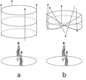
III.1.9 As the drum major in Figure 20 now marches around her identity, S’, she creates a set of circular n, m, and p bounds for the emerging and rectilinear nm, np, and mp they form. That circulation, no matter what its dimensionality, can now be the one-manifold that acts as the foundation for a set of biological-ecological transformations.
Whitney (1940) first properly defined the terms now in common use. In his terminology, the drum-major’s traverse is acting as a “base space”. He referred to the baton that she takes up as “fibre”. And if she holds her fibre over her base space as she walks, then she creates a “fibre bundle”. It is the product of two contributory topological spaces.
Fibre bundles create a conjoined XY topological space that allows us to draw conclusions about the original X and Y. If, for example, our X base space is the globe of the earth, while the Y fibre is the wind velocity at each point, then the resulting XY fibre bundle allows us to conclude—in line with algebraic topology’s “hairy ball theorem” that there is no non-vanishing continuous three-dimensional tangent vector field on an even-dimensional n-sphere—that there is always some point where wind velocity is zero.
III.1.10 The one-manifolds that are our base spaces and fibres can easily have different dimensionalities. Their interaction will then certainly be homotopically equivalent, but need not be homeomorphic. The fibre bundles that two different populations or generations can each create can only be homeomorphic if the dimensionalities of each of their bases and fibre bundles match.
Just as the drum major’s base space can oscillate using x⁄x’, so can the fibre potentially oscillate as y about y’. However, if we ensure that our fibre always stays the same side of its y’—such as when a tree grows from a minimum to a maximum, and does not itself return to any minimum, thus always being +dx; or when a sperm cell swims and depletes its mass-energy, without fertilizing to return to a maximum, so always giving -dx—then our baton or fibre is the line segment Y = [0, 1].
Since our base space is X = S1 for a circle; while the baton or fibre is Y = [0, 1] for a line segment; then the bounded x region, upon the projective plane and/or Möbius strip must be a trivial cycle. The x region, supporting that y, is an orientable disc formed about a rotahedron’s surface. It does not cross a hemisphere. That limited and bounded x region will—as a homeomorphism—be a region of discrete biological activity. As a homomorphism, it will be a set of ordinary nonreproductive metabolic-physiological processes undertaken by the entities. It will only move from preimage to image or vice versa; and/or from replication to biology globe or vice versa; but it does not undertake both transitions, for it does not have both recurvature points. It does not cross the replication point and so does not complete a generation.
As in Figure 20a, this limited fibre bundle, created as X × Y, will be a cylindrical x × y bundle that again does not reach from boundary to boundary. Such fibre bundles can contribute to either a fibration, θ, or a cofibration, ρ, but not to both.
III.1.11 As in Figure 19b, the three two-manifolds τtn, τtm and τtp are critically different. They all contain τt. They can freely therefore cross the equator and pass through both identification points. By Meme 89, since each individual manifold in these latter couplings, with t, maintains its distinct identity, then they can both at some times be less than each of their respective identities; they can both at other times be greater; or one can be greater while the other is less; and vice versa. They are two-braids that exhibit the closure of a braid, and so can return to their start points for a generation. Since they contain t they have the global topologies that wrap around to create a circulation of the generations.
III.1.12 But if two-manifolds are indeed going to wrap around for a generation, then they must still abide by certain constraints. By Meme 90, we can relate the two components directly to each other. One will then at some point be greater than the other; and at other times it will be less. The two therefore see-saw about each other in two overall regions. Their two-braid thus creates Figure 19b’s “braid-2” with those two flip orientations. But their combination—as they cross the projective plane and curve about the circulation—is always some S; the sum of their changes is still ∫dS = 0; and their overall equilibrium is still some S’.
III.1.13 We now add the extra constraint, seen in Figure 20b, that a recurvature point exists. The drum major now twirls the baton with sufficient acceleration to range y both sides of y’. As she marches, our y now oscillates about its midpoint, and goes through its own complete revolution in conjunction with x. The point of recurvature will occur when the rates of change of latitude and longitude, relative to the surface, are zero.
We have here a different X × Y product. Suitable initial values plus rates of change mean the drum major carries this fibre right across the projective plane. Both base and fibre can now return to their start points for a generation. The baton’s recurvature or inversion is the constraint that creates the fibres that can then participate in nontrivial fibre bundles.
We now have a Möbius strip: the simplest nontrivial example of a fibre bundle. It has the lifting property that allows it to provide both fibrations and cofibrations with its recursive functions. The recurvatures help create the curvilinear point-, line-, realm-, and tetraspaces that are the biovolumes, V, that drive all biology. It crosses both the replication point and the generation bound.
III.1.14 For Meme 91, we next conjoin the manifolds in threes. They form the four 3-balls, realms, and rotahedrons τtnm, τtnp, τtmp and τnmp.
By Meme 92, all the four rotahedrons can create realms whose local topologies and fibre bundles are flat, featureless, and Euclidean. They have the familiar three dimensions of left-right, front-back, and up-down, or (x, y, z).
However, the τnmp rotahedron is different from the other three. It is again without t. It can only access Euclidean properties. So by Meme 93 it cannot recurve any of n, m, or p about a circulation; and it cannot create nontrivial fibre bundles.
By Meme 94, the three remaining rotahedrons—τtnm, τtnp, and τtmp—all contain τt. They can all recurve globally to form realmspaces. Over their whole cycle, however, one component will sometimes be greater than the others; sometimes less; and sometimes in between. The three interact to form biological parallelepipeds whose side lengths see-saw about a cube, producing both the three-braid and the “braid-3” shown in Figure 18c. They establish the accelerations and values for nm, np, and mp at each point in a generation. When one of its three components either increases or decreases, the other two must flip to either decrease or increase to maintain equilibrium. This gives six flippable orientation regions of greater and lesser inequalities. The sum of all their joint realmspace changes is still zero … and a joint S’ equilibrium again exists.
III.1.15 And finally, Meme 95 brings all four one-manifolds together. The fourth splits each of the six braid-3 regions to give a constant t-acceleration. This draws all local and global topologies together to create an overall four-manifold and rotachoron tetraspace of τtnmp. This creates a four-braid and a “braid-4”. It is a “four-parallelotope” whose side lengths see-saw about a tesseract. This gives 24 regions—such as t > n > m > p—navigated in regular succession for both S and S’, with various dimensional flip orientations and permutations to create a rotachoron. Since t is present in them all, then n, m, and p recurve about each other to form a circulation.
These t-accelerations in the various τtnmp configurations are now responsible for all terrestrial biology. They establish the values for nmp—and a braid-3—all about the circulation; as also for each of them again in their different configurations throughout all three- and two- manifolds, both homomorphically and homeomorphically. If any of n, m, or p are considered biological, then both their recurve or generation length T, and the population that contains them, must be specified. That is the recursive biological function and process that uses the nucleotide codons of DNA to create all circulations of the generations specified by the t in τtnmp.
III.1.16 Our τt, τn, τm, and τp manifolds therefore behave as follows:
• The τn, τm, and τp in isolation have each been flattened from some higher dimension of τtn, τtm, and τtp, and carry n, m, and p values measured in the surroundings at that given time t, and at that point in the overall circulation. The one-braid and braid-1 give them a constant state maintained as dτ/dt.
• The τnm, τnp, and τmp have also each been flattened from τtnm, τtnp, and τtmp and therefore possess a constant acceleration to keep exhibiting those values all about a circulation. The two-braid and braid-2 carry them through their values from minimum to maxiumum and returning as d2τ/dt2.
• The τnmp has been flattened from τtnmp. This then carries the nmp all about the circulation. They get their values from the three-braid and braid-3, as d3τ/dt3.
• The whole is maintained by the governing S3–V4 rotachoron that establishes the overall biology and ecology of λ, and through the θ fibration and ρ cofibration.
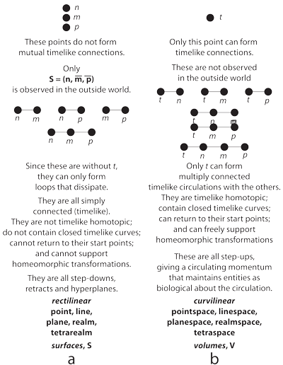
III.2.1 Figure 21 now confirms Meme 88. When our n, m, and p manifolds are independent of t, then as in Figure 21a, they cannot create circulating biological-temporal momentums. They must instead move rectilinearly. Since the τt manifold does not accelerate them hyperspherically about the circulation of the generations, they can only form “spacelike” structures. Those are without t. They again ray out through surfaces upon the rectilinear ijk axes. They become measurable, in the surroundings, with SI units, as the various observed biological constructs, and obey the second law of thermodynamics.
III.2.2 Meme 96 then specifies, as in Figure 21b, that when n, m, and p are accelerated about the circulation by the τt manifold, they associate with t in some hyperspherical biovolume, V. The only way to measure them is through some biological population, V, that encloses them within some set of biological structures, S. That population has then used its recursive functions as a language of syntax and semantics to create the necessary nucleotide codons.
Each of the n plessists that the τt and τn manifolds form bind their distinct Ingredients 3 and 4 stocks of p and m. Those can then undertake their metabolism and their physiology as infinite cyclic groups, complete with infinite generators, and infinite cyclic subgroups through γ, ψ, and λ.
III.2.3 If the plessists formed by the τt and τn manifolds are to reproduce, they must recurve. They must form wind walls. But they must also be biological. They must survive for the time TN—which is the circulation length τn—so they reach the replication point. They can then be observed using their cofibrations and their nontrivial fibre bundles to reproduce.
A biological circulation can only exist, at every moment τ0t0, when there is a positive number, n, of plessists. The circulation as a whole must therefore have ∫dn ≥ 0.
III.2.4 Each of the n plessists that exists at any time can only, by definition, contribute to its τ circulation for as long as it accelerates hyperspherically. When each has ∫dp < 0 and/or ∫dm < 0, then each is by definition trivial and without t. Each can only dissipate. So if each is to recurve and be a generator, then each must satisfy ∫dp ≥ 0 and ∫dm ≥ 0.
III.2.5 Since each individual plessist in a reproducing population must have its distinct stock of p for its plemes, and so that ∫dp ≥ 0, then there immediately exists a population energy, P, that satisfies:
P ≡ np̅,
where p̅ is the average individual value over the population, along with a suitable distribution.
III.2.6 There must also be a joint population mass M, plus distribution, satisfying:
M ≡ nm̅,
where m̅ is now the average individual components value, as their plessiomes, plus its distribution.
III.2.7 For every population value P and M, then there are by definition n plessists, each of p and m for its plemes and plessiomes. But these n plessists can now always be substituted for by their n plessemorphs. There are always—and by definition—n such in any plessist population, demonstrating the right helicoid behaviour. This is all so by definition, and in our model.
III.2.8 For every n plessists we immediately have a shared value p̅ and m̅ and a population P and M constructed equally by those plessists and their archetypal plessemorphs. The m̅ defines the plesseomes for each of the n plessemorphs. And since it is two-dimensional, it exhibits a surface that supports a recurvature. In the same way, the p̅ defines the distinct plessetopes for those same archetypal n plessemorphs, as the surface supporting the same recurvature.
III.2.9 We note, for Meme 97, that all our population’s measurable properties, S, for those plessists and their plessemorphs, must now be given, through those same plessemorphs, by:
S ≡ (n, m̅, p̅).
III.2.10 By Meme 98, then at every moment all about the circulation, which is for every τ0t0 between τ-1t-1 and τ1t1, our plessemorphs are described, in terms of the plessists they substitute for, by p̅ = P⁄n and m̅ = M⁄n. These must always exist, along with their infinitesimal plesseome and plessetope increments of dm̅ and dp̅. This is again so by definition.
By Meme 99, the population’s instantaneous change at any time is given by:
dS ≡ dn + dm̅ + dp̅.
III.2.11 We have already met the above as the braid-3 of Figure 19c. And since the population identity S’ can only be preserved when dS’ = dn’ + dm̅’ + dp̅’, then when any one of n’, m̅’, or p̅’ leaves that equilibrium value, then at least one of the other two must move in the opposite direction to restore it. That net dS’ interaction must now define the dt = Tdτ equilibrium that is the biological activity λ at every point. It characterizes the plessemorphs and their plesseomes and plessetopes that in their turn create the 1s for the doubly closed equilibrium that define π.
III.2.12 And … by Meme 100, this is all a Lorentzian four-manifold. Those sub-manifolds without τt can only form simply-connected timelike loops that can use their embedded Hooke cell and deformation retract of (n’, m̅’, p̅’) to lift as fibration, θ, from image to mapping cylinder, or else as cofibration, ρ, from preimage to mapping cylinder. Each is also either a λ journey from image to preimage as progeny codomain to progenitor domain; or else from preimage to image as progenitor domain to progeny codomain.
The submanifolds formed with τt are multiply-connected timelike. The entities formed can now use the same (n’, m̅’, p̅’) Hooke cell and deformation retract, embedded in them, to recurve. They can eventually undertake the inverse transitions of both ρ cofibration and θ fibration that lift from both preimage and image to the same mapping cylinder, creating the complete biological–ecological interactions, λ, for a generation.
III.2.13 We now have both the homomorphisms and the homeomorphisms that describe any group of plessists. We can also identify m̅ with γ, and dm̅’ with dγ; and p̅ with ψ, and dp̅ with dψ. But … these are precisely the components in our Whitney umbrella.
III.2.14 And since M = nm̅ then if ever n stays constant M and m̅ must have changed at the same rate over some interval, T. The same goes for P = np̅.
III.2.15 We indeed have n = M⁄m̅ = P⁄p̅. This means that if ever the population values M and P change at a different rate from the individual values m̅ and p̅, then numbers, n, must be changing. And … this is very easy to measure. It was indeed the basis of our entire Brassica rapa experiment.
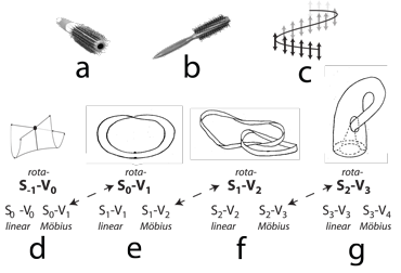
III.3.1 The realization that two or more of our distinct dimensions can combine to act as a single one-manifold is highly problematic. As in Figure 22, biological entities have three modes of presentation. It is why we cannot yet define a species. Those random manifold and dimension combinations allow the homomorphic to be merely homotopically equivalent without being homeomorphic.
III.3.2 By Meme 101, although our homomorphisms can demonstrate their equivalence by being locally indistinguishable, they are our biological structures centred upon points. Our homeomorphisms are—by contrast—the specific recurvature–capable transformations maintained by these homomorphic and so fully replicative biological structures. But whether our interactions are merely homomorphic or more specifically homeomorphic, they will involve both (a) the points that are the individual homomorphisms and structures, and (b) the entire groups of points that are then the homeomorphisms as the spaces being occupied.
III.3.3 Again by Meme 101, our homomorphic biological structures reside in those topological spaces called manifolds. A manifold’s properties mean that every point in any homomorphic neighbourhood—which is a biological structure—will always appear locally Euclidean, while globally being otherwise. The structure can now globally either simply dissipate; or else successfully remain biological and transform via the replication globe. But they will appear the same, locally.
III.3.4 Since our biological manifolds can have different dimensionalities, then they are, locally, some collection of the real numbers, ℜ. The number of different real numbers we need to represent any given biological structure depends upon that dimensionality, n. So if some biological homomorphism uses n distinct sub-manifolds, then we can easily track its biological homomorphisms with some ℜn. This simply means a collection, n, of coordinates which are real numbers, ℜ.
III.3.5 Fibre bundles are instead based on entire neighbourhoods … i.e. they are constructed from entire groups of points, and not simply from points. Like the two hairbrushes in Figure 22a and b, a fibre bundle involves three different topological spaces, each of which is in our case a manifold. We have (i) the base, B, which can be a first homomorphic structure, and which on the hairbrush is its underlying cylinder; (ii) the fibre, F, which can be either the surroundings or another manifold, and is the hairbrush fibre; and (iii) their product space P = B × F, which is the hairbrush’s overall shape.
The fibre bundle now means that every neighbourhood, or small region, of P will look like whatever is the composition, B × F, of both base and fibre. That product space is their local neighbourhood coordination of points.
Our fibre bundles can track all our homeomorphisms, which are the effects our two homomorphisms have on each other and on the surroundings. They can do so on their joint product space, P. Each P can then use a “projection map”, ξ, to map continuously back to each of its B and F components … but so that it has a continuous surjective, or onto, function, ξ(p) = b, which maps from P to the base space, B. So if we begin at some p in P, such as the tip of some hairbrush fibre in Figure 22a, then we can project along the fibre, back down to embed b in B. For every point b in B, there is at least one point p in P.
III.3.6 However, we could in fact have created a product space that is instead a Möbius strip, such as with the twisted hairbrush in Figure 22b. But unfortunately, the projection ξ(p) = b along the fibre back to the base works just as well as it did in the straight hairbrush in Figure 22a. This means that the points p in our product space P can easily have attributes not originally present at any b in B. Fibre bundle neighbourhoods can clearly have extra properties not present in either base, B, or fibre, F. We cannot therefore define species as proposed groups, because they will exhibit recurvature behaviours different from any of those possessed by their members, but in unpredictable ways.
III.3.7 A circle as base, and a line segment as fibre can create either a cylinder or a Möbius strip for their fibre bundle. But all neighbourhoods in both the resulting cylinder and the Möbius strip will still be locally indistinguishable. Either way, we get our embedding into the base. We can now easily have our semantic and/or syntactic comprehension capability, in our product and fibre bundle, but with one or another of the aphasias. The information from either the base or the fibre necessary to fully access the product space need not necessarily arrive.
III.3.8 Figure 22c also shows that a line segment taken as the fibre to a circle, for its base, can potentially produce a “tangent bundle” that appears, locally, as an infinitely long straight line, U. The tangent bundle is some “open set”, U. This simply means there can be infinitely many different ones, of infinitely many types, but all tangential. Each open set appears, locally, as U × ℜn.
III.3.9 Figures 22d, e, f, and g, and their Meme 101 tell us that (i) the rectilinear Euclidean, (ii) the circular, and (iii) the twisted Möbius fibre bundles are all locally indistinguishable. Figure 22d tells us that our S-1–V0 pointspace—which builds all biology—is a Whitney umbrella bounded by -r and +r input-output points. These can circle outwards and return to pass through the same point, but with opposite properties, so manifesting a V0 pointspace. But it can all the time act, to the surroundings, with a flat S0 unchanging Euclidean local topology. A given cell can have the same inertia whether it is a parent, or is busy splitting into two daughters.
III.3.10 A population can only complete a circulation if it and its entities exhibit a constant acceleration to carry them about some recurving wind wall. The components must undertake whatever transformations will return them to the beginning of a generation, τ.
III.3.11 These three possibilities—the linear, the circulating, and the twisted—mean that any two S0 points can bound an S0–V1 line with a flat Euclidean S1 local topology. The resulting curving linespace and global topology can bound a V2 planespace. That S1–V1 line could also however be the S0–V1 unknot with crossing, of Figure 22e. It can then bound what looks distinctly like an S1–V2 rotagon. It now has the extra dimension, and so can acquire a crossing.
We can use any S1–V1 line or linespace to curve about and form an S1–V2 rotagon. This again has the local topology of a flat and unending Euclidean plane, but the global topology that bounds a V2 planespace. But we can just as well produce that same infinitesimally local planespace by travelling infinitely often about the S1–V2 Möbius strip of Figure 22f. The result is indistinguishable from either a rotahedron’s infinitely surrounding S2 manifold surface upon an S2–V3 rotahedron; or from an infinitely extended Euclidean plane.
We can in the same way create an S2–V3 rotahedron with a flat and infinitely extended plane for its surface that is entirely consistent with an infinitely extended S3 Euclidean local topology for a realm; but that nevertheless has the global topology of an ever-curving three-dimensional realmspace. But we can get that same V3 realmspace by going indefinitely about the surface of a Klein bottle as an S3–V4.
III.3.12 If our drum major now takes up a zero-dimensional point and uses an S1 marching circle as her base, then she creates an identical S1 circle for her fibre bundle. But since the point is locally rectilinear and Euclidean, it is a value maintained invariantly over time. And further since it is accelerated about the circle that is its base, it forms a trivial cycle upon a rotahedron. It bounds a region.
III.3.13 We now add the extra constraint that our drum major twist that point as she marches. This is the Whitney umbrella and its S0–V0 transformation as the point seemingly journeys between -r and +r in its pointspace, demonstrating first one then the other, so being first an input, and then an output, while all the time maintaining its absolute value, |r|. It is now carried all about a generation.
The fibre bundle is no longer a trivial cycle. It instead becomes an unknot with crossing. It can participate in a recurvature.
III.3.14 We now have the two globally curving neighbourhoods formed by a “0-ball” as fibre, at a given distance from a circle as base: one with twist, and the other without. The former’s twist means it can switch from +x to -x and so cross a real projective plane. The latter cannot.
III.3.15 If the drum major next takes up a line segment as a fibre—which is some property’s journey outward from its minimum to its maximum, or else conversely—then her marching produces a cylinder as fibre bundle. And if we again add the twisting constraint, to allow the value to move to the other side of an identity and to return to its initial value to complete a circuit, then we again have a recurvature. Some single value can both increase and decrease while others remain the same. We have a Möbius strip. These are the two neighbourhoods formed by a 1-ball as fibre, at a given distance from a circle as base, under both constraints.
III.3.16 And if the drum major now takes up a circle as fibre—which is an entire two-dimensional interaction and so surface—and holds it vertically to march about, then she creates a torus that can be a set of trivial cycles maintained over time. And if she twists it as she walks, then the cycle of increments is some ±dA that creates a Klein bottle. That recurvature is a 2-ball as fibre a given distance from a circle as base under both constraints. We now have a nontrivial cycle that can be the base for a generation.
III.3.17 And, finally, if she takes up a sphere as fibre and marches, then she creates a “spheritorus”, which is energy and work trivially maintained over time. And if she twists it, the three values have a joint ±dV to create a higher-dimensioned Klein bottle. The same work and energy can now fuel a generation. These are the two neighbourhoods formed by a 3-ball as fibre, at a given distance from a circle as base, under both constraints.
III.3.18 Fibre bundles hold the spatial properties of entire groups of points. They can appear, locally, as homeomorphic to both their bases and their fibres, while having global properties distinct from each. The two together are the biological interactions, λ. They form the various homomorphic S-V structures which can then interact with different homeomorphisms with the surroundings.
We can now track all deformations between preimage and image, and between the biology and replication globes, as both bases and fibres. Whether as manifolds, or as fibre bundles, they will all be homotopically equivalent. But only some will be homeomorphic. If we want to allocate different entities and groups to diferent species, then we must distinguish their different syntactical and semantic combinations, as DNA nucleotide codons, to form the various possibilities that are all locally Euclidean, but globally distinct.
III.3.19 If we do not clarify these differences then we will never identify the different species.
III.4.1 A biological population and/or its generation can now be a fibre bundle. This will be some arrangement of our four manifolds or dimensions.
III.4.2 Although the V4 rotachoron, complete with its S3 or three-dimensional glome surface, that we use to represent a population, remains impossible to display in the two dimensions on a piece of paper, Manning (1914) showed that it nevertheless remains accessible to thought. As in Figure 23, a dimension is any value or property capable of demonstrating some independent change.
As with our fibre bundles, any two dimensions taken together can alter with respect to each other, and immediately form a surface. Our Frenet-Serrat trihedron promptly makes all their mutual rates of change accessible.
III.4.3 Just as an S2 planespace can have (a) the completely flat local topology of an infinitely extended plane, which means no changes in some aspect or dimension; yet (b) is also the surface bounding a V3 rotahedron, which means regular infinitesimal and linked changes in others; while also (c) potentially expressing the twist of being carried about a Möbius strip, which means oscillating back and forth about a mean; then so also does each S3 that is a bounding glome upon a V4 rotachoron have (a) the local topology of an infinitely extended rectilinear realm or three-dimensional space; (b) the global topology of a realmspace that curves about a V4 surface; and (c) the twist of a Klein bottle. This again simply means the dimensions—even when largely conceptual—have different ways of changing with respect to each other, both locally and globally.
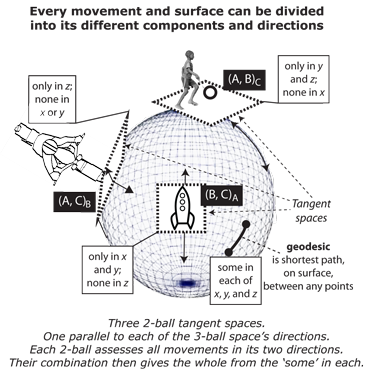
III.4.4 As again in Figure 23, an ordinary V3 rotahedron is any set of properties, (A, B, C) we can describe using its three S2 “tangent spaces”, one parallel to each axis, and so as (A, B)C, (A, C)B, and (B, C)A. Holding one specific direction constant allows us to analyse movements in the others.
III.4.5 The same principle applies to the four dimensions or properties in our V4 rotachoron. This is an (A, B, C, D) that has four perfectly ordinary 3-ball Euclidean S3 glomes—one parallel to each direction—acting as its flattening and surface tangent spaces. These are (A, B, C)D,
(A, B, D)C, (A, C, D)B, and (B, C, D)A. ‘Straight’ then simply means the path whose “tangent vectors” are currently running parallel to some selected axis. We simply note all values and changes while some specified one holds constant.
III.4.6 If we take an (A, B, C) rotahedron, then we can first consider the (A, B)C surface. This is the same as a two-dimensional being observing a series of concentric circles as the rotagon pushes up, through his or her universe, which is his or her flat AB plane (Abbott 1884). The circles he or she sees will grow from an infinitesimally small size to a maximum width—which is the sphere’s diameter—and then back to a minimum as the sphere pushes right through his or world, and through his or her plane. If the sphere does the same for the other two (B, C)A and (A, C)B possibilities, which are pushes in the A and B directions, then the two-dimensional being can observe the entire rotahedron. This is the same principle, for ourselves, in our three-dimensional world, as we contemplate a four-dimensional (A, B, C, D) rotachoron. It has four-directions in which it can push through our world.
III.4.7 A rotahedron’s three S2 planes combine as the three 2-ball flattening Euclidean planes. We observe it as the familiar curving exterior. And just as those three S2 planes combine to create a rotahedron’s surface … then so also do the four S3 glomes upon a V4 rotachoron’s surface combine to produce its overall three-dimensional realmspace as its surface. This is then observable as an apparently ordinary Euclidean realm or infinitely extended 3-space … except for additionally exhibiting the biological events that tend an entire population from generation beginning to end. That is then the fourth dimension’s curvature. We observe this curving as the waxing and waning of the generations, and as some set of dτ events about a global circulation, for every absolute and linear dt in time. We have dt = Tdτ, with T = 2r being the radius of curvature.
III.4.8 There is one further—and very important—consideration. The spherical wheel pushing up from underneath the hoop runner in Figure 23 has the same single osculating contact point as the cylindrical one he pushes down from above. The hoop runner confirms that the S2-V3 rotahedron underneath him is also a spherical wheel rolling upon his tangent planar surface.
We can always replace the sphere—as the hoop runner above does—with a cylinder, or hoop, of arbitrary length. The sphere is then identical, at its contact point, to the hoop runner’s cylindrical wheel above. That cylinder can then turn to roll in whatever direction. The sphere’s movements are now exactly replicated, on that tangent surface, by that cylinder, which in its turn gives the impression of being able to roll infinitely far in any direction on that surface.
III.4.9 Our Frenet-Serrat trihedron can now isolate all axes and 1-balls to find the biological “geodesic”. This is any population’s straightest—and so shortest—local path in a biological landscape. It is a movement with respect to our biology and replication globes, and our progenitor domain and progeny codomain. This can then be expressed in terms of the patterns and behaviours displayed by the nucleotide codons existing at any point, and as they instantaneously transform to others.
III.4.10 And now we have characterized both the structures and the spaces, we can describe all biological entities and their entire ecological behaviours.