IV.1.1 We now return to our Chomsky grammar to find the genetic–linguistic production rules that emulate our fibre bundles. They must separate our replicative recurvatures and our Möbius strip transitions across identified boundaries from mere biological-metabolic trivial cycles. We must be able to distinguish all (x, y)α biological perspectives and observations from all (x, y) nonbiological ones, where α is some coupling such as wz that recurves.

We therefore reaffirm, for Meme 102, that although the homomorphic objects making up our preimage and image have access to a vast number of transformations, they are made from a limited and countable number of Ingredients 3 and 4 that are always equipollent with ℵ0, the set of countably infinite natural numbers. Those laws, maxims, and constraints, working over four dimensions, are then the inheritable transformations that render them biological.

IV.1.2 Noam Chomsky proved (1956)—in solving a very similar problem—that grammar is the study of the infinite expressions we can produce, using finite means. He thus linked the infinite expressiveness of language, which is the ability to produce infinitely many sentences, to automata theory, when seen as the study of the infinite possibilities of self-acting devices, again using finite means. Since grammar has become the study of the differences between recursive functions and loops, then it is also the study of the differences between semantic interiors and syntactic surfaces.

IV.1.3 By Meme 103, although the local, the global, and the Möbius strip behaviours that our biological structures engage in always appear the same locally, we can distinguish them using both (a) the Chomsky(–Schützenberger) hierarchy, and (b) the “Church–Turing thesis” (Copeland 2000). These together separate recursive functions from loops.

IV.1.4 The Church-Turing thesis says that anything we can do with a set of recursive functions, we can also do with a series of loops. We can understand the important difference between them by proposing that I want to track down my old primary school friend Gnowee. Since I do not know her number, I call Anowah. She also does not know it, but says Boakye does. So I call Boakye, who tells me to try Chandra … who proposes Dagvald … who refers me to Euan … who at last suggests Fareeha who at last gives it to me. I could potentially go on indefinitely, asking as many as necessary. I have personally undertaken six iterations of the ‘do-it-by-yourself’ loop.

But if, now, Anowah were instead to offer to call Boakye for me; and if she passed back the information; and if Boakye offered to do the same for Anowah; and if all others emulated that behaviour when approached; then that would be six recursive ‘let-me-do-that-for-you’ function calls. This could also go on indefinitely. The end result is the same, for I still get the information. But in the loop case, I have to make all calls myself (one to each and every person in the chain); whereas in the recursive function case, I—personally—only have to make the one (I only need to call Boakye).

IV.1.5 Chomsky then proved that even though recursive functions and loops have a complete equivalence, a loop-only grammar must nevertheless become prohibitively complex … whereas a recursive function based one can produce the infinitely many outputs in any language—even of arbitrary complexity—by stepping through a far simpler set of very basic constructs.

IV.1.6 Our Meme 103 therefore uses both the Church-Turing thesis and the Chomsky hierarchy to turn biology into the study of the infinite possibilities of the infinitely many self-perpetuating and homomorphic entities composed from the finite means of the radiative and the circulating Ingredients 3 and 4. They then behave homeomorphically, with respect to our two identified boundaries.

IV.1.7 Biology has thus become a bioinformatics study. It is the study of the homotopically equivalent transformations between progenitor domain as preimage; and progeny codomain as image; and conversely; using deformation retracts and mapping cylinders, along with manifolds, fibre bundles, and fibrations and cofibrations as they shift between our biology and replication globes.

IV.2.1 We have already defined the entirety of the λ biological-ecological behaviours over a generation as both (a) the mapping cylinder, Mλ; and (b) an infinite cyclic group. The fibration and cofibration, θ and ρ, are then the complementary operators that can produce the infinite cyclic subgroups using the biological grammar of Figure 24a. The elements in the group are our plessists and plessemorph. They are formed by ψ and γ, themselves composed from Ingredients 3 and 4 as a result of θ and ρ and their interactions with the surroundings.

IV.2.4 The V2 surface in Figure 24b displays one aspect of our biological grammar. It is acting as a “flattening agent”. Any (x, y, z) construct in Figure 24a can use any direction to flatten as (x, y)z etc.

More generally, and in our topological grammar, any lower-dimensioned Sn-1 object can act as a “hyperplane” that flattens some immediately higher Vn dimension onto any of its Sn-1 surfaces. As with Figure 24b’s rotahedron becoming a bounded rotagon upon that plane, that Vn object is becoming a Vn-1 ball surrounded by an Sn-2 surface. We thus declare this aspect of our grammar, for Meme 105, by saying that the intersection of every n-ball with its retract n-1 hyperplane produces an n-1–ball. We can produce each object in Figure 24a using this method.

IV.2.5 There is, however, a converse aspect to this grammar. Every n-ball can be an n-sphere that surrounds. That flat V2 surface in Figure 24b is a small portion extracted from a rotahedron of infinite radius. It then acts as the surface that cuts into—and so establishes—an interior and an exterior, and/or lesser and greater, for a higher-dimensioned n+1 ball of radius r. So if we assign ‘0’ to the cutting hyperplane, then everything in V3 to one side of V2 is ‘greater than’, the other side being ‘less than’. We can again both produce and describe each object in Figure 24a using this method.

IV.2.6 But a Vn always has an Sn-1 bound. As with the rotagon on the surface in Figure 24b, the Vn’s surrounding n-1–sphere can be the “trace” that creates that n-ball by establishing some radius r. That n-ball is then a union of concentric n-1–spheres of volume Vn and surface Sn-1. That n-ball is thus the similar trace, whose union of concentric n–spheres produces a sphere of volume Vn+1, for which it is the surface Sn.

IV.2.7 Figure 24b shows our grammar in action. The way the film in a camera “step-down retracts”. or flattens, a three-dimensional view down to only two, is similar to the retractions of a two-dimensional V2 rotagon to a one-dimensional S1 line segment or unknot; and also of a V1 line segment down to its two S0 points separated by 2r. Those various step-downs create loops which pass outwards, through those surfaces, into the surroundings. They can, however, also be fibre bundles with an added twist.

We have here an example of our multidimensional syntax and semantics. We select some value or statement x’, establishing a sequence of statements as a radius r, and creating the hyperspherical boundary, τ, that is the biological language. It is simultaneously:

• a journey about a helicoid;

• a trip across a real projective plane;

• a circulation about a rotahedron; and

• the Möbius journey about a set of self-intersecting Whitney umbrellas.

IV.2.8 But if biological entities are to survive, then recursive functions, and step-ups, creating cofibrations and biovolumes, must exist. So if, as in Figure 24b, we push a V3 rotahedron through a V2 world, that step-up process will look—to the inhabitants—like a two-dimensional rotagon steadily growing from a minimum width; to its maximum; and diminishing back to its minimum (Abbott 1884). Since the inhabitants can deduce the rotahedron that has passed through, we have reversed the above flattening process.

IV.2.9 All such step-ups are our recursive functions. The resulting S1–V2 biosurface is perceived as the waxing and waning of an S2–V3 biovolume, and so as a dynamic biological cycle.

And then just as we can use an architect’s two-dimensional plans as a trace to construct a three-dimensional house, so also is a square pushed upwards through a plane the trace for a cube; and so again is a plane’s above sequence of concentric circles the similar trace for a sphere. We can even allocate a central point as a zero; establish lefts and rights, or insides and outsides; and separate that higher-dimensioned object into two. The dimensionality of any resulting Vn+1 is always one greater than the dimensionality of whatever hypersphere allows that Vn to be a trace; and that can also flatten or divide the resulting Vn+1.

IV.2.10 For Meme 106, we take time, t, as the fourth dimension. We can then take up an entire V3 or three-dimensional realmspace. We use it as a trace to create step-ups, reversions, and recursive functions as we push it through our fourth-dimension to produce a tetrarealm by waxing and waning, in time, as both a self-intersection, and a complete circulation of the generations. It is the tetraspace and biovolume, V4. It is the transition from progenitor domain and preimage to progeny codomain and image, and back.

IV.2.11 It is impossible to display the resulting V4 rotachoron plus its S3 bounding glomes upon a piece of paper’s only two dimensions. But we can observe biological entities waxing and waning as they are carried about their circulation, which is through a generation, τ. That τ is then the time that it takes to push or flatten a biological rotachoron through this three-dimensional realm. We simply use t as a hyperplane to create a biological tetraspace that can only be observed over time, and as the cycle of birth, development, reproduction, and dissipation.

IV.2.12 Our biological Chomsky grammar is now the fibration, θ, plus cofibration, ρ, using the deformation retract, S’, to lift to the surrounding mapping cylinder, Mλ … all as the observable biological processes, λ. The structures are manifolds and homomorphisms. The processes are fibre bundles and homeomorphisms. Both involve ψ and γ as the language of the Ingredients 3 and 4 of photons and molecules.

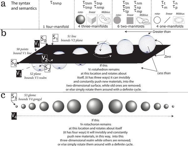
IV.2.13 As in Figure 24a, we can use a recursive function to draw Ingredients 3 and 4 in from the surroundings. This creates the four one-manifolds, six two-manifolds, four three-manifolds, and the single four-manifold that we cannot show in two dimensions, and that is the S3–V4 rotachoron. That rotachoron can then be flattened with any one of the four different hyperplanes t, n, m and p to produce the four glomes of τnmp, τtmp, τtnp, and τtnm respectively.

IV.2.14 The nmp glome has a special status in this grammar. It is a triple set of terminals. All this glome’s products and constructs loop out into the surroundings.

IV.2.15 The remaining three τtmp, τtnp, and τtnm glomes can each again be flattened, with hyperplanes, into different directions to produce the six curving τtn, τtm, τtp, τnm, τnp, and τmp two-manifolds that are their surfaces.

IV.2.16 The three surfaces without t—nm, np, and mp—again have a special status and are terminals. They therefore loop out into the surroundings.

IV.2.17 And, finally, the remaining three τtn, τtm, τtp surfaces are then further flattened upon the t hyperplane to produce the values for n, m, and p. These are terminal values observed at those specific points τ in the circuation … which is also at some definite and terminal moment of absolute clock time, t.

IV.2.18 Biological entities and materials are thus the spoken syntax and semantics of nucleotide codons within this bioinformatics grammar.

IV.3.1 Chomsky again proved (Chomsky 1956; 1959) that when a finite set of resources is combined with a limited set of rules, it can nevertheless produce infinitely many objects. Our grammar is that every Vn biovolume is also an Sn biosurface to some Vn+1, whilst itself being bound by some step-down Sn-1, which is itself a Vn-1 biovolume bound by its own Sn-2 biosurface … and so on down to distinct S0 input–output points.

Our chosen language only needs to span across S0,1,2,3 and V1,2,3,4. This is three transitions between the biologically and replicatively closed and open, which is between the non-injective and the injective, the non-surjective and the surjective. They are our three constraints.

IV.3.2 As in Figure 21b, every biologically infused n, m, and p—which are our Ingredients 2, 3, and 4—must at some time link to t, our Ingredient 1, to become timelike connected; produce the timelike homotopic circulations that support homeomorphic transformations; and form the closed intersecting timelike curves that can return to their start points for a generation, τ. Elements without τt retract by taking t as their hyperplane. They are relinquished to the surroundings as loops. These are indistinguishable from the tail recursive functions and τn, τm, and τp that drive them.

IV.3.3 Our Chomsky grammar is therefore now that every biovolume as some cell, entity, species, or terrestrial Gaia principle is a step-up composed of recursive functions involving τt; while its every presenting biosurface of molecules, genomes, gene pool and entire collection of terrestrial DNA is the equivalent step-down, composed of loops in n, m, and p at some absolute clock moment, t. With three such t-constraints upon n, m, and p in place, then our biovolumes formed from recursive functions can fly away from the circulating τt to deliver themselves, to the surroundings, as loops.

IV.3.4 Our τn, τm, and τp manifolds are one-dimensional unknots. They increment about the closure of their braid. They move from S-1 to S1 all about their identity, S’. Ingredients 2, 3, and 4 must thus undertake their transformations over τn, τp, and τm to match τt. But these are also the absolute time spans TN, TP, and TM that the plessists—and therefore plessemorphs—take over a generation.

IV.3.5 Since the population of plessists must recurve about our globes, then it must meet the following three constraints:

• We have carefully defined our nn plessists so they always act exactly as a population formed by their na archetypal plessemorphs would also act. Since they are both composed from both of our radiative and the circulating field principles, then this Ingredient 2 of n must be the least variable of the three. And since all the n plessemorphs must—by definition—recurve about both our globes, then they must at a minimum satisfy ∫dn = 0 for our first constraint.

• Each of the above n plessists and their plessemorphs must be composed of a discrete number, m, of molecules. Since component numbers can remain constant even as chemical reactions rearrange chemical bonds within any given entity, then this is the next most variable. Its recurvature about the same globes is given by ∫dM = 0 as our second constraint.

• The population energy, P, as the radiative principle, must be the most variable of the three for any p in any individual n can change as both n and m hold constant. It must abide by ∫dP = 0 as our third constraint.

IV.3.6 Those three properties of ∫dn = ∫dM = ∫dP = 0 are the three constraints to which all biological populations must be subject. Populations must allocate entities to the replicatively and/or biologically closed and/or open, and to trivial and nontrivial cycles, according as to whether they do, or do not, return to each globe; and also according as to whether they are, or are not, injective and/or surjective. But if populations are to circumnavigate both globes and complete a generation, then they must abide by the above constraints that establish the recurvature conditions.

Since biological entities and populations must recurve about our globes, then the sum of the transformations in any viable population must once again be ∫dn = ∫dM = ∫dP = 0. And if any population is to remain stable, then those transformations must also satisfy ∫dS’ = 0. This general grammatical rule of ∫dn = ∫dM = ∫dP = ∫dS’ = 0 therefore defines the fully biological-ecological DNA and nucleotide codon grammar. These are the “exact differentials” that establish the recurvature parameters.

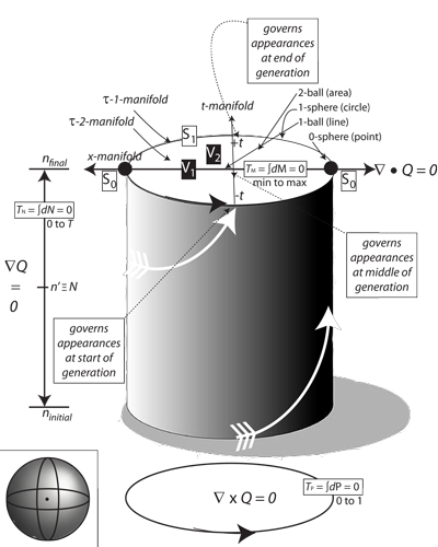
IV.4.1 Although four dimensions cannot be properly displayed in only two, Figure 25, which is Meme 106, nevertheless attempts to portray the fuller implications of each of the four S3–V4 rotachoron diameters. It suggests the behaviours of one of the four, which is thus acting as a Hooke cell would act in creating a dynamic equilibrium. This is to maintain an S’ deformation retract state using its S0 inputs and outputs. Those +r and -r exchanges provide the driving forces that produce measurable external results.

Figure 25 may look static, but it is again a set of dynamic events occuring at real and measurable speeds over each of its four diameters. The dynamic equilibrium is a set of constant and precisely balanced interactions with the mapping cylinder and surroundings.

As with the three-dimensional rotahedron equilibrium represented at the bottom of Figure 25, the four directions combine to project towards a central point. Just as those three circles create a rotahedron by intersecting and moving about each other, so do their four four-dimensional equivalents similarly intersect to create a rotachoron. All four diameters deformation retract to the same central point, which then establishes the radius, r, for them all.

IV.4.4 While an ordinary three-dimensional cylinder is bounded by two two-dimensional circles at each end, the spherinder is bounded by two spheres or 3-balls at each end. And when that ordinary cylinder pushes, with its flat side first, through an S2 plane, then the plane’s two-dimensional inhabitants detect a circle of unvarying size passing by them over some given time interval T that is the cylinder’s length. But if it is pushed through with its round side first, then they will see a line that grows to a rectangle, and then goes back to a line. In the same way, when a four-dimensional spherinder is pushed through our three-dimensional S3 realm with its “flat side” first, then we will detect a sphere of constant dimensions pass by over some time T, that is its length; and if it is pushed through with its “round side” first, then we will see a complete cylinder that similarly grows and shrinks from a line back to a line.

IV.4.5 We can create the biological spherinder for a generation by projecting a sphere across the line of length T, which is then its axis. But since a spherinder is a diameter, then it can trace out a rotachoron by turning about itself in exactly the same way that either a two-dimensional circle or a cylinder can create a sphere by rotating about. The rotating spherinder’s beginning and end points are then coincident. They self-intersect. When we leave one spherical face, we automatically reenter through what looks like the opposite face, at the other end, but we in fact keep going with the same spherinder, continuously, in the same direction about the surrounding rotachoron. Therefore, if the spherinder’s two ends are the same size, then we have both a uniform rotachoron and an infinitely long Euclidean line. It and its centre are the four-fold stationary S4–V4 point … and state the recurvature properties.

IV.4.6 A point or infinitesimally short line segment can create a diameter by pushing all across a rotagon; and a point or infinitesimally small circle can create a diameter by pushing across a rotahedron. Since an infinitesimally small rotahedron can similarly create our spherinder by pushing diametrically across the rotachoron, then a spherinder is the fibre bundle we construct by projecting a V3 rotahedron, as a fibre, along a line segment, which then acts as a base. The spherinder is therefore the infinitesimally thin cross-section across the V4 rotachoron’s 2r = T diameter. A part of its length is the fibration; a part is the cofibration. A part is therefore the biology globe, a part the replication one. And further since a spherinder has spherical and self-intersecting ends, then it forms a closed loop. It endlessly restates the same biological interactions, generation after generation. All points in our rotachoron become glomes; all lines—particularly the four diameters—become spherinders; and all planes—particularly the τnmp one that defines all real-world behaviours—become infinitesimally thin cubinders. A spherinder therefore defines our unipollent and doubly closed equilibrium, π.

IV.4.7 Since a biological circulation is exactly a recurvature, as a return to an original state, then our spherinder can also be thought of as an infinitesimally short section along a spheritorus … which is itself the fibre bundle created by projecting a V3 rotahedron, as a fibre bundle, about a circle of diameter T and radius r acting as a base. The spherinder is then taken along the “hypercircumference” τ. Events now enter and leave the spherical volume elements, at each end, all about the circulation. Their properties again state the recurvature at every point.

IV.4.8 Every present moment τ0t0 in Figure 25’s spherinder lies between τ-1t-1 at the beginning of a generation and τ1t1 at the end. Every τ0 exists within some curvilinear interval τ-1–τ0–τ1, while every rectilinear moment t0 occurs within some rectilinear time interval t-1–t0–t1. Every present population state S0 transforms between S-1 and S1. Therefore, every absolute and rectilinear time interval dt along the spherinder’s interior axis is a part of the generation length T; but it is also always accompanied by some curvilinear interval dτ about the spherinder’s exterior as a part of the circulation of the generations, τ. These together are the dt = Tdτ that define the successive points a, b, and c upon a helicoid, a rotahedron, a projective plane, our Möbius strips and the like.

IV.4.9 Since there are the four manifolds and directions of t, n, m and p, then there is one such spherinder in each direction, and along each axis. The n direction with its ∫dn = 0 may be the least variable of the three constraints by defining the number of plessists, but their contribution to any S at any point can still change by dn. The two respective rates of change will be dn⁄dt along the spherindrical axis, and dn⁄dτ about its surface and the boundary, which is the circulation length.

IV.4.10 We first introduced, in Meme 99, the mean across any interval, along with its distribution, as n’. We now further define that mean, for Meme 107, as “one biomole”, N, where:

n’ ≡ N.

So if the number of plessists across any interval is ninitial at one end and nfinal at the other, then the number of plessemorphs maintained across that same spherindrical interval is immediately n’ = N = 1 biomole where n’ is the weighted mean. This simply confirms that our n plessists can define our archetypal plessemorphs, and conversely. The number maintained across any spherinder is therefore N … while the number at the centre for the deformation retract of any ninitial and nfinal is also n’ = N. Meme 108 then says that any population maintaining its mean across any spherindrical interval has a size of N = 1 biomole of plessemorphs … while still behaving in the identical way as the n plessists concerned.

IV.4.11 Meme 109 then further says that any population maintaining its N = 1 biomole mean for 1 second has a “numeracy”, Q of, for example, “one biomole per second”. This is simply a way of saying that the population is, at that moment, maintaining its average numbers for that interval. A numeracy less than 1 means the population has proportionately less than its average number for that interval; and conversely if Q > 1.

IV.4.12 As again in Figure 25, Meme 110 now confirms that the absolute population number at the edges of any interval are ninitial and nfinal. Meme 111 then formally identifies the absolute time TN along the axis with the matching circulation distance τn; and similarly with TM and τm, TP and τp, and T and τt. This is effectively to say that we have four spherinders in four different directions across our rotahedron, all of which are equivalent in sharing the same central point as their deformation retract.

IV.4.13 Since our absolute time interval across the spherinder has the limits 0 and T, then the number of plessemorphs across our spherinder, in the n direction, and for those limits, is:

N = ∫Q dt.

The numeracy at each point across the spherinder is then:

Q = dN⁄dt.

IV.4.14 We are again expressing numbers in terms of the mean across whatever interval. And then since that same interval has the limits 0 to 1 for the curvilinear interval, τ, then the same population of plessemorphs must exhibit that same equilibrium, between those limits and be observable in the outside world as:

N = ∫Q dτ.

and:

Q = dN⁄dτ.

IV.4.15 By Meme 112, the gradient in numeracy across the spherinder, ∇Q, is the rate at which the population numbers, of whatever absolute size, must either increase or decrease to attain and maintain the mean for each over that interval. It is:

∇Q = (nfinal - ninitial)⁄N.

But since we currently have ∫dn = 0, then the gradient across our spherinder, and for an entire generation, is zero; as also is the rate of change of gradient. And … if ever both the gradient in numeracy and its rate of change across any interval are zero, then we have a static dynamic equilibrium, and that population is “numerically static”. This is the “stasis of the first kind”.

IV.4.16 A stasis of the first kind is a dynamic equilibrium determined not just by the number of plessists, but by the number of plessemorphs we can substitute for them. Whatever the plessist numbers at either end of the interval, they collapse infinitesimally smoothly into the N plessemorphs that are their centre and the deformation retract. This stasis of the first kind is the first requirement for our defining self-intersection and unipollent equilibrium, π.

IV.4.17 These are, however, biological entities. Their numerical stasis, as plessists, is not possible without some kind of (A) plessiome and (B) pleme interaction, in the surroundings, to support it. These involve the mapping cylinder, Mλ, and therefore a specified stock of chemical components and joules of energy. There must also be plesseomes and plessetopes for our plessemorphs.

IV.4.18 There are again four manifolds, one for each of our Ingredients. The m direction is the next most variable of the three constraints. It acts in conjunction with the n direction to establish ∫dM = 0 over the population.

This dynamic equilibrium requires that when we look in the m-direction, we see an equilibrium number of components flowing past each edge of the same interval. Those quantities must emulate N and come smoothly and infinitesimally into a mean at the centre to create the deformation retract. The n plessiomes must form the N plesseomes for our plessemorph gene pool.

No matter what their -r and +r exchanges, these S0–V0 pointspaces have the constant values for n, m and p at each t. By our Meme 104 Chomsky grammar, our population is now constructing a homogeneous V4 rotachoron of fixed and maximum volume with radius, r, in its four directions of t, n, m, and p. All V0 pointspaces must have the overall S0 point behaviours whose exteriors produce the local topology of an infinitely long and one-dimensional Euclidean line at each distinct t all about every circulation. And since our self-intersection demands that r is constant in every direction, then:

n2 = m2 = p2 = t2 = r2,

which in its turn defines:

τn = τm = τp = τt = τ.

All our four one-manifolds now have the same two solutions of +r and -r imposed by their deformation retract. All four therefore exhibit the same S0 = -r and S0 = +r points all about the V4 rotachoron. As in Figure 25, our equilibrium occurs when the amount of biological processing, dτ, in any absolute interval, dt, is always the same, both relatively and absolutely, so that dt = Tdτ; and so that our rotachoron preserves its total V4 gongyl.

The rotachoron’s four τtnm, τtnp, τtmp, and τnmp bounding glomes are also the rotahedrons that hold the S2 surfaces that create the dt = Tdτ. Each bounding surface therefore holds the interactions that are the external biological–ecological presentations. They produce both π and the sequence of equilibrium-creating 1s. But this again means all V0 pointspace inputs and outputs all about the circulation, when summed, have matching inputs and outputs over every Whitney umbrella.

Since this is already a numerically static population, then by Meme 113, the spherinder in the m-direction must help create both ∫dn = 0 and ∫dM = 0. These define its surrounding cubinder upon the rotachoron surface. We can therefore determine the divergence in the components that preserve the above self-intersection and dynamic stasis in numeracy.

If both the population numeracy and the plesseomes must remain the same across this interval, then the same numbers of components must again flow in and out of the spherinder to give a divergence of zero. The divergence in the plessiome and plesseome components that construct our plessists and plessemorphs is therefore:

∇ • Q = m̅final - (m̅initialninitial ⁄nfinal)

Both the gradient and the divergence are now zero, ∇Q = ∇ • Q = 0. The population is maintaining both those means across an entire interval. Its rate of change must also be zero right across the spherinder, with the central point again being the deformation retract. So if ever both (a) the divergence, and (b) its rate of change are zero, then the population is “materially static”. This is the “stasis of the second kind”, and is the second requirement for our full unipollent equilibrium.

IV.4.19 If these first two directions are indeed dynamically static, then so also must be the one for our plemes and plessetopes, which is our third and final constraint of ∫dP = 0. Every spherinder, in every direction, must therefore sit centrally in its surrounding cubinder which is its specified contribution to the mapping cylinder, Mλ. The time across this third spherinder is TP. The net Ingredient 3 interaction must satisfy TN = TM = TP = T and τn = τm = τp = τ which are, respectively, the diameter and the circumference.

Since the population gradient and divergence are already both zero, then the curl must match the gradient and divergence so that exactly the same amounts of energy enter and leave the plessist population and each plessemorph at each moment. Therefore any two subpopulations A and B must sit evenly either side of their shared equator and prime meridian, forming a squaroid to give both dtAB = TABdτAB, and ∇Q = ∇ • Q = ∇ × Q = 0. But… this is the Hooke cell … our deformation retract … and our identity, S’.

Since the gradient, divergence, and curl are all zero, then all τtn, τtm, and τtp pairings will act as 1-spheres to V2 rotagons; with each having the local topology of an infinite flat Euclidean S2 plane or surface. All V2 rotagons are the S2 planespaces whose curls drive the circulation, bounding the observed V3 rotahedrons which are the waxing and waning of biological activity.

And … we have successfully described the rates of interactions with the surroundings that produce our π equilibrium. The Ingredients 3 and 4 that construct our plessemorphs across the interval ninitial to nfinal, must jointly satisfy:

∇ × Q = Pfinalm̅initial - Minitialp̅final
= p̅finalm̅initial(nfinal - ninitial).

When both this curl and its rate of change are zero, then the population is “energetically static”. This is the “stasis of the third kind”, and the third requirement for our plessemorph’s unipollent equilibrium, π.

IV.4.20 With the stases of the first, second, and third kinds we have now defined the conditions that allow any infinite cyclic group population with a biology and ecology of λ to create its infinite cyclic subgroup behaviours of ψ and γ so it can produce the recurvatures that allow it to traverse a Möbius strip and complete a generation, so constructing its biological equilibrium. That equilibrium is S’, which is also the deformation retract, or generation centre point, of S’ = (N, m̅’, p̅’) held at some specified τ’t’ which is both the middle of a generation in absolute clock time, and its centre as a distance. This then constructs the mapping cylinder, Mλ, all about itself as the surroundings. That is the complete set of interactions for a generation.

IV.4.21 Each of the three values in the deformation retract is held at its independent point in the generation at its t0, which is also some absolute clock moment t in the overall generation length, T. The three nevertheless conjoin as the infinitesimally small self-intersecting sphere that is also the fibre stretching across T, as its base, to construct the four spherinders that are the population’s four V4 rotachoron diameters. And since S’ = (N, m̅’, p̅’) is the deformation retract; and also since all infinite cyclic groups are equipollent with the additive group of integers; then S’ states the closed, static and unipollent behaviours that can indifferently substitute for any population in all its activities.

IV.4.22 A spherindrical population, complete with its fibration and cofibration of θ and ρ, and its deformation retract of S’, all active across T, are both the syntax and the semantics that construct the λ that are the mapping cylinder’s biology and ecology. They are the surrounding fibre bundle and cubinder of τ. All populations can then use their DNA syntax and semantics to oscillate about the three kinds of stasis of ∇Q = ∇ • Q = ∇ × Q = 0. They are the stases of the first, second and third kinds, being the numerically, the materially, and the energetically static, for the deformation retract.

IV.4.23 But the populations simultaneously apply the three constraints of ∫dn = ∫dM = ∫dP = 0 over that T to create the recurvatures around our biology and replication globes that are the manifest biological entities engaging in their activities to construct a generation.

IV.4.24 This Meme 112 therefore defines a biological population as one that satisfies both (a) the three constraints, and (b) the stases of the first, second, and third kinds.

IV.5.1 Our population of plessists and plessemorphs must now create both (a) the three kinds of stasis of ∇Q = ∇ • Q = ∇ × Q = 0; and (b) the three constraints of ∫dn = ∫dM = ∫dP = 0. They each use the Chomsky production rule of [Σ, S, δ, α0, F] to create the needed biological structures and behaviours.

IV.5.2 All viable populations must create a specific biology of syntax and semantics. Their various recursive functions must accept molecules from the surroundings through S0 acting as inputs, and convert them into their various biological entities. Those nucleotide codons, genomes, and other structures will be the V1,2,3,4 biovolumes and energies as step-ups and sequences of fibrations and cofibrations. They will manifst as S0,1,2,3 structures, jointly imposing their recurvatures as biological events. We therefore need a series of production rules that set δ to some value.

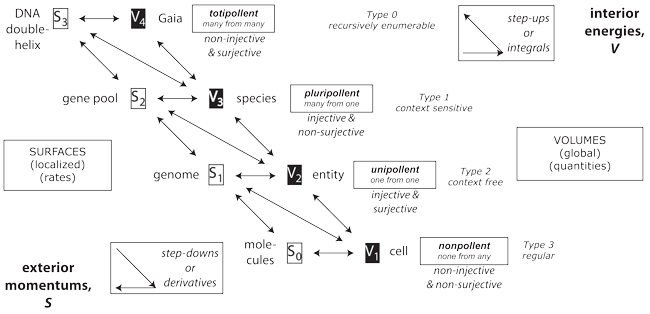
IV.5.3 For Meme 113, we note that, as in Figures 1 and 26, when the four levels Lloyd discusses (2012) are understood as the four combinations of mappings of injective and non-injective, surjective non-surjective between sets of progenitors and their progeny, then they correlate precisely with the “Chomsky hierarchy” (Chomsky 1956; 1959). The biological cycle occurs because the same step-up materials that a Chomsky production rule builds as V1,2,3,4 semantic productions immediately loop outwards into the surroundings, through S0 outputs, and courtesy of the second law of thermodynamics, as observed constructs and biosurfaces, and so as step-downs and S0,1,2,3 syntaxes. The δ in [Σ, S, δ, α0, F] must therefore step through those levels so that the constraints and their recursive functions—based on fibrations and cofibrations involving θ, ρ, ψ, and γ—will create the spherinders and their surrounding cubinders that define our biological equilibrium, π.

IV.5.4 Meme 114 now sets our Chomsky input alphabet to the four nucleotide “letters” of the DNA codon alphabet. This gives Σ = {A, C, G, T}. Our start symbol, α0, is always then some initial set of codons that is also some S-1 = {n, m̅, p̅} as a preimage in a progenitor domain.

And … we straight away procure a stoichiometric index (BIPM 2006) into the DNA alphabet. Since our Chomsky and Church-Turing grammar over this language—with its recursive functions of our fibrations, cofibrations, and the like—can rearrange those letters into all possible DNA strings, then they are the gateway to all 20 amino acids, and so to all possible proteins and biological entities.

IV.5.5 Our recursive function’s initial string is some α0 = {A, C, G, T}, which is again S-1 = {n, m̅, p̅} as a preimage in a progenitor domain. An RNA production uses its recursive function to transcribe the amino acid language, using the surroundings as a mapping cylinder, so inducing a set of λ biological activities. Since they are processes involving n, m̅, and p̅, then the resulting terminal string takes the form F = {A, C, G, T}; while also giving some final S1 = {n, m̅, p̅} as an image in a progeny codomain..

IV.5.6 The recursive functions in our Chomsky production drive the multiply connected timelike circulations τtn, τtm, and τtp. Since these all involve t, the functions create the surfaces and collections of nucleotide codons. Their multiply connected and higher-dimensioned productions are τtnm, τtnp, τtmp, and τtnmp. They ultimately use t as a hyperplane to flatten themselves into their final values n, m, and p at some moment. As given Chomsky production rules, these products are therefore the results of recursive functions created from those same nucleotides, all flattened with a t hyperplane to become nm̅, np̅, m̅p̅, and S = {n, m̅, p̅}.

IV.5.7 For Meme 115 the first result in our Chomsky production is the nonpollent S0-V1 level of molecules–cells. But when those nonpollent productions leave the replication globe and enter the biology one, they do not return. The best they can do is form a set of trivial cycles.

Our nonpollent entities have a fibration, but no cofibration. They do not cross the projective plane. We can denote this by saying that they have a “reproductive index” of δ = 0. They therefore have a Chomsky production rule of:

[Σ={A, C, G, T}, S = {n, m̅, p̅}, δ = 0, α0, F].

IV.5.8 Our nonpollent entities may not reproduce, but this above production rule can nevertheless produce infinitely many of infinite variety … as many as there are sentences in any spoken language. Their lack of ability to reproduce is not specific to any Kingdom; nor to any entity.

Complete nonpollent entities could perhaps be a set of pre-Archaea entities. Those likely had no nucleus, and no membrane-based organelles. We do, however, have worker ants, worker bees, mole-rats and other such strictly eusocial entities as cannot reproduce. We also have nonreplicative parts contained within entities, such as our own neurons. All such nonpollent biological materials, wherever located, are equivalent to Chomsky’s Type 3 regular grammars, and so to fixed finite state automata.

IV.5.9 Meme 116 gives our second Chomsky production. This is the unipollent level of S1-V2 and genome-entity. This is not merely single-celled entities. It covers any biological material—i.e. in or out of any entity or population, and within any Kingdom—that can replicate.

These unipollent entities do not support trivial cycles, but can re-enter the replication globe. They are equivalent to Chomsky’s “Type 2” or “context-free grammars”, and so to ‘pushdown automata’. Since they can reproduce, we allocate them a set of fibrations and cofibrations with an index δ = 1.

IV.5.10 Our next Chomsky production of Meme 117 produces the third pluripollent level of S2-V3 gene pool–species. This is all biological materials—again wherever located—that can both (a) replicate, and (b) support at least some material(s), that cannot. They are suitably exemplified by asexual multicellular entities such as polyps, flatworms, and anything that can bud, fission, and engage in vegetative reproduction, as do starfish that can regenerate from cut limbs. They are also such constructs as organs and tissues. These are produced by trivial cycles in the biology globe, but must be replicated by some nontrivial one that crosses the projective plane. They are equivalent to Chomsky’s “Type 1” or “context sensitive grammars” representing ‘linear bound automata’. We set their δ to any integer value.

IV.5.11 Meme 118 is our final totipollent production level. This S3-V4 is DNA-Gaia. We set the reproductive index, δ, to any positive, but non-integer, value.

These productions characterize biological materials produced of more than one reproductive centre. Although they can go through trivial cycles in the replication globe, they must always be supported by some nontrivial one that carries them across the projective plane. They are equivalent to Chomsky’s “Type 0” “unrestricted grammars”; are recursively enumerable; and embrace sexual reproduction of:

π = (2 × 1½ → n)1 ⇔ (n ÷ 1½ → 2),

where δ is set to ½.

IV.5.12 We have now accounted for all biological materials. We have a progenitor domain as preimage and progeny codomain as image. Their recursive functions are mappings that are either injective or non-injective; and either surjective or non-surjective.

IV.5.13 Our last task is to categorize these productions. They are all homomorphic and homotopically equivalent. But some are additionally homeomorphic.

IV.5.14 We are at last ready to find the rules for the stases of the first, second and third kinds of ∇Q = ∇ • Q = ∇ × Q = 0 and that are also the three constraints of ∫dn = ∫dM = ∫dP = 0. These separate the injective from the non-injective, and the surjective from the non-surjective. They thereby also separate preimage from image, and the progenitor domain from the progeny codomain to create all biological entities and behaviours.